SLAM Accelerated Using Hardware to improve SLAM algorithm

SLAM Accelerated Using Hardware to improve SLAM algorithm performance

Project Overview ¡Team Members ¡ Roy Lycke ¡ Ji Li ¡ Ryan Hamor ¡Take existing SLAM algorithm and implement on computer ¡Analyze Performance of algorithm to determine kernels to be accelerated in HW ¡Implement SLAM algorithm on Power. PC with previously identified kernels in HW RH

What is SLAM? ¡SLAM stands for Simultaneous Localization and Mapping ¡ Predict pose using previous and current data ¡ Types of pose sensors ¡ Wheel Encoders ¡ GPS ¡Detect landmarks and correlated to robot using predicted pose. ¡ Types of Observation Sensors ¡ Sonar ¡ Infrared ¡ Laser Scanners ¡ Video RH

Current State of SLAM Algorithms ¡SLAM algorithms fall into two main categories ¡ Extend Kalman Filter ¡ Large Covariance Matrix to Process ¡ Particle Filter ¡ Each Particle contains pose estimate and map RH

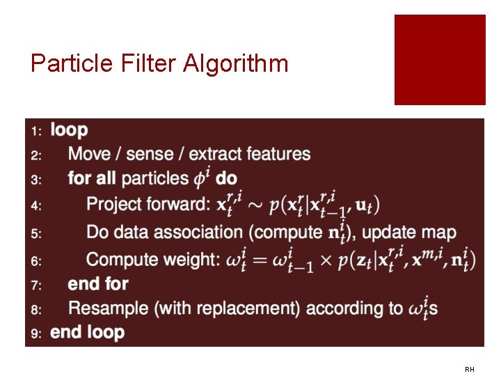
Particle Filter Algorithm RH

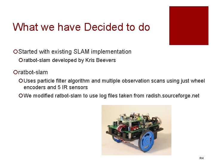
What we have Decided to do ¡Started with existing SLAM implementation ¡ ratbot-slam developed by Kris Beevers ¡ratbot-slam ¡ Uses particle filter algorithm and multiple observation scans using just wheel encoders and 5 IR sensors ¡ We modified ratbot-slam to use log files taken from radish. sourceforge. net RH

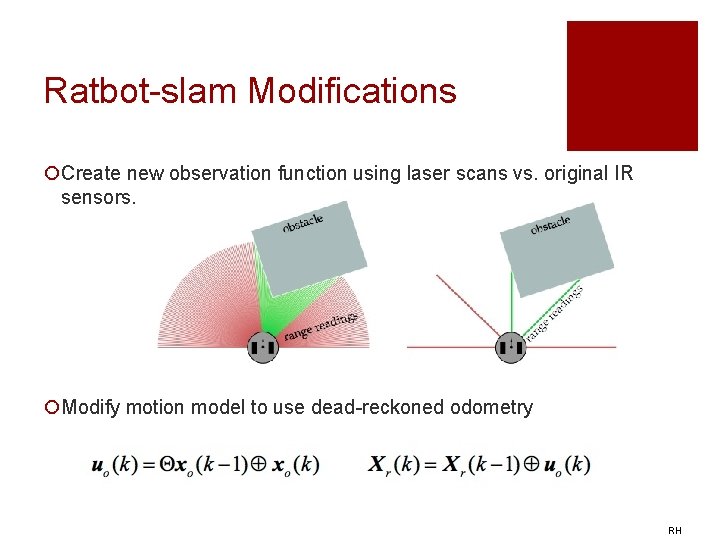
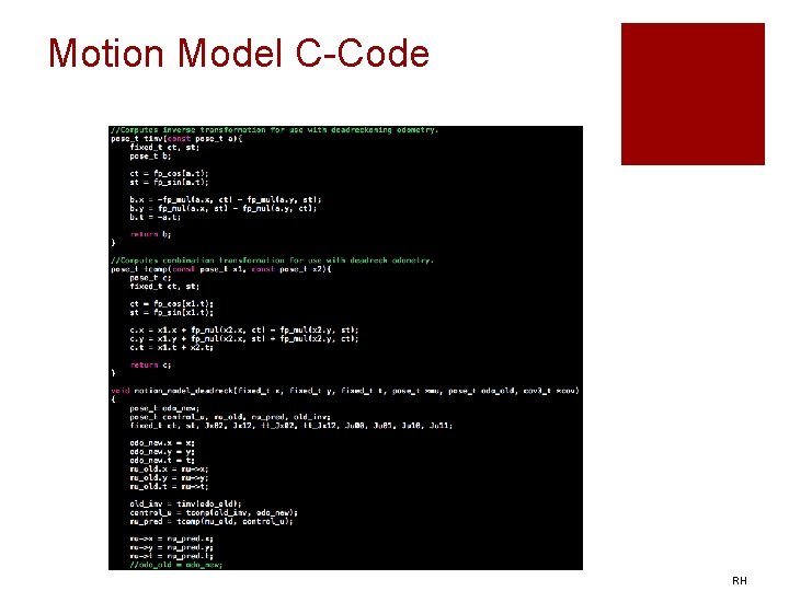
Ratbot-slam Modifications ¡Create new observation function using laser scans vs. original IR sensors. ¡Modify motion model to use dead-reckoned odometry RH

Demo of Modified ratbot-slam RH

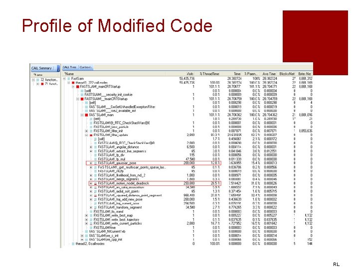
Profile of Modified Code RL

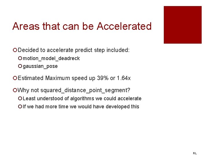
Areas that can be Accelerated ¡Decided to accelerate predict step included: ¡ motion_model_deadreck ¡ gaussian_pose ¡Estimated Maximum speed up 39% or 1. 64 x ¡Why not squared_distance_point_segment? ¡ Least understood of algorithms we could accelerate ¡ If we had more time we would have developed this RL

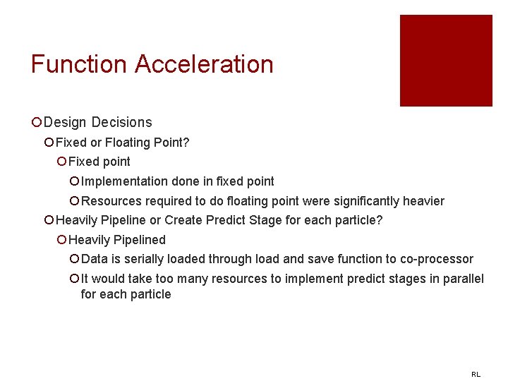
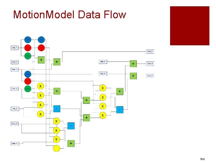
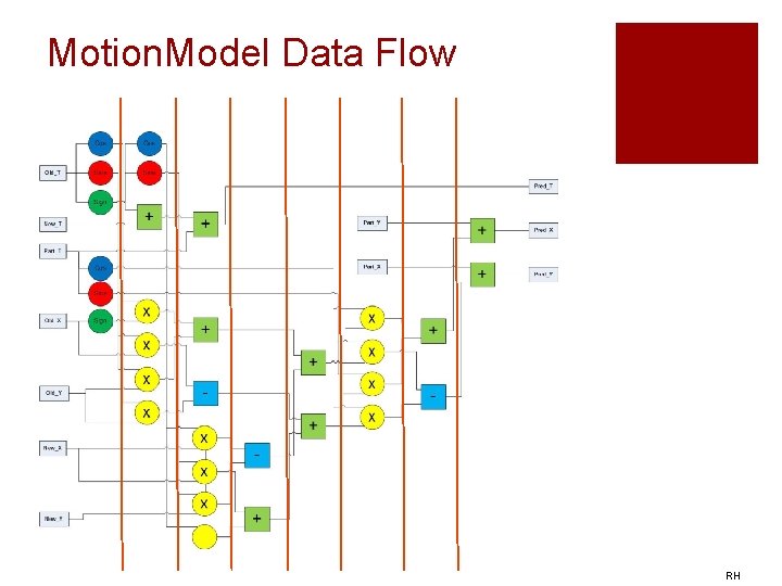
Function Acceleration ¡Design Decisions ¡ Fixed or Floating Point? ¡ Fixed point ¡ Implementation done in fixed point ¡ Resources required to do floating point were significantly heavier ¡ Heavily Pipeline or Create Predict Stage for each particle? ¡ Heavily Pipelined ¡ Data is serially loaded through load and save function to co-processor ¡ It would take too many resources to implement predict stages in parallel for each particle RL

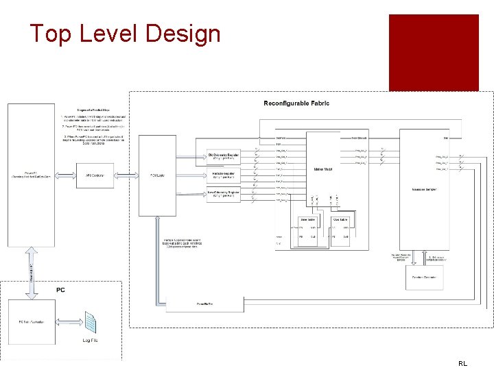
Top Level Design RL

Motion Model C-Code RH

Motion. Model Data Flow RH

Motion. Model Data Flow RH

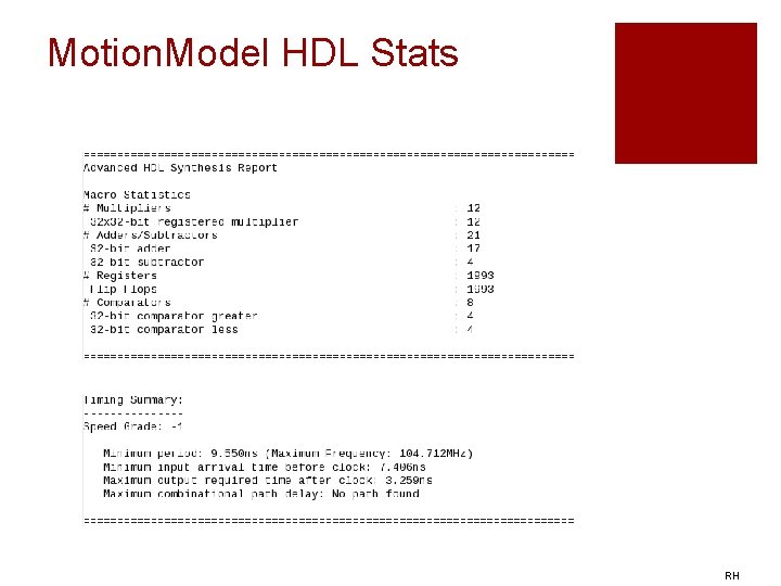
Motion. Model HDL Stats RH

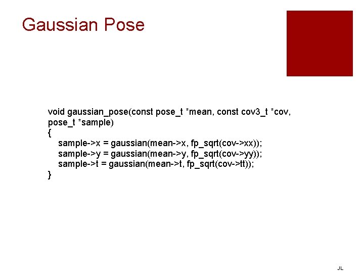
Gaussian Pose void gaussian_pose(const pose_t *mean, const cov 3_t *cov, pose_t *sample) { sample->x = gaussian(mean->x, fp_sqrt(cov->xx)); sample->y = gaussian(mean->y, fp_sqrt(cov->yy)); sample->t = gaussian(mean->t, fp_sqrt(cov->tt)); } JL

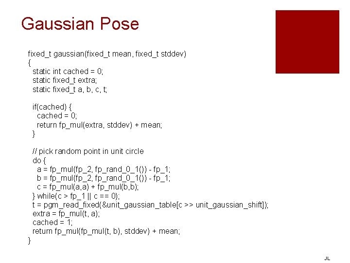
Gaussian Pose fixed_t gaussian(fixed_t mean, fixed_t stddev) { static int cached = 0; static fixed_t extra; static fixed_t a, b, c, t; if(cached) { cached = 0; return fp_mul(extra, stddev) + mean; } // pick random point in unit circle do { a = fp_mul(fp_2, fp_rand_0_1()) - fp_1; b = fp_mul(fp_2, fp_rand_0_1()) - fp_1; c = fp_mul(a, a) + fp_mul(b, b); } while(c > fp_1 || c == 0); t = pgm_read_fixed(&unit_gaussian_table[c >> unit_gaussian_shift]); extra = fp_mul(t, a); cached = 1; return fp_mul(t, b), stddev) + mean; } JL

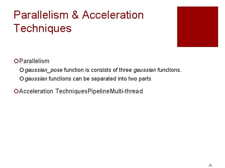
Parallelism & Acceleration Techniques ¡Parallelism ¡ gaussian_pose function is consists of three gaussian functions. ¡ gaussian functions can be separated into two parts ¡Acceleration Techniques. Pipeline. Multi-thread JL

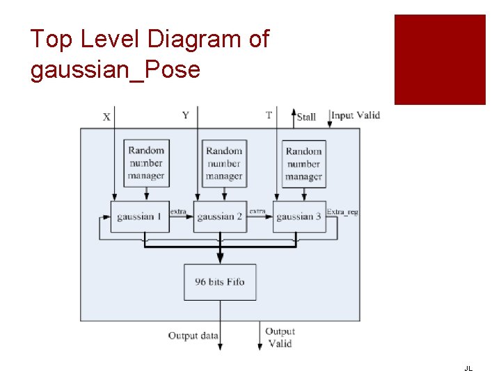
Top Level Diagram of gaussian_Pose JL

Random Number Generator ¡Xorshift random number generators are developed. They generate the next number in their sequence by repeatedly taking the exclusive or (XOR) of a number with a bit shifted version of itself. JL

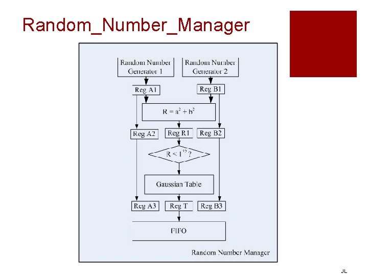
Random_Number_Manager JL

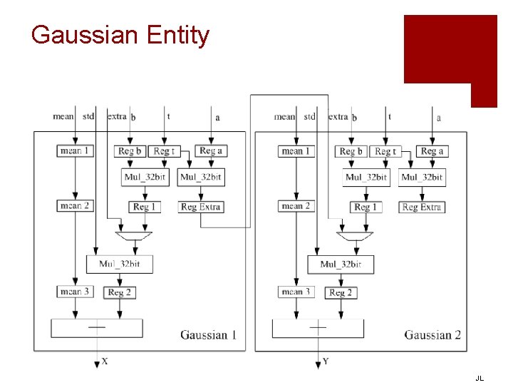
Gaussian Entity JL

Demo of FPGA System RL

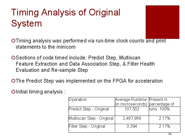
Timing Analysis of Original System ¡Timing analysis was performed via run-time clock counts and print statements to the minicom ¡Sections of code timed include: Predict Step, Multiscan Feature Extraction and Data Association Step, & Filter Health Evaluation and Re-sample Step ¡The Predict Step was implemented on the FPGA for acceleration ¡Initial timing analysis : Operation Predict Step - Original Multiscan Step - Original Filter Step - Original Average Runtime Present in (in microseconds) percentage of runs 100% 107, 502 2, 487, 969 2. 17% 3, 394 2. 17% RL

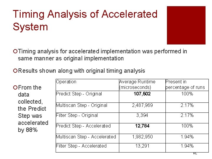
Timing Analysis of Accelerated System ¡Timing analysis for accelerated implementation was performed in same manner as original implementation ¡Results shown along with original timing analysis ¡From the data collected, the Predict Step was accelerated by 88% Operation Predict Step - Original Multiscan Step - Original Average Runtime (microseconds) 107, 502 Present in percentage of runs 100% 2, 487, 969 2. 17% Filter Step - Original 3, 394 2. 17% Predict Step - Accelerated 12, 784 100% 1, 982, 950 1. 94% 13, 291 1. 94% Multiscan Step - Accelerated Filter Step - Accelerated RL

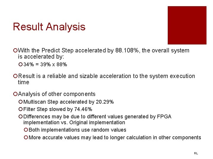
Result Analysis ¡With the Predict Step accelerated by 88. 108%, the overall system is accelerated by: ¡ 34% = 39% x 88% ¡Result is a reliable and sizable acceleration to the system execution time ¡Analysis of other components ¡ Multiscan Step accelerated by 20. 29% ¡ Filter Step slowed by 74. 46% ¡ Differences may be due to different values generated by FPGA implementation vs. Original implementation ¡ Both implementations use random values ¡ More accurate values may lead to longer calculation in other components RL

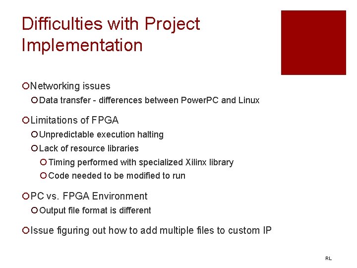
Difficulties with Project Implementation ¡Networking issues ¡ Data transfer - differences between Power. PC and Linux ¡Limitations of FPGA ¡ Unpredictable execution halting ¡ Lack of resource libraries ¡ Timing performed with specialized Xilinx library ¡ Code needed to be modified to run ¡PC vs. FPGA Environment ¡ Output file format is different ¡Issue figuring out how to add multiple files to custom IP RL

Conclusions ¡Based on the run-time analysis of our implementation of the accelerated SLAM algorithm there was an appreciable speed up achieved. ¡Our Implementation achieved a speed up of approximately 34% or 1. 51 x out of an ideal 39% or 1. 64 x ¡This result shows that if more of the SLAM algorithm was implemented on an FPGA there could be a greater acceleration. ¡Top issue in SLAM implementations is getting algorithm’s implemented on embedded real time systems RH

Future Directions ¡Add more regions of the Algorithm to the FPGA acceleration ¡ Current implementation only accelerates 39% of system ¡Run SLAM system on different FPGA ¡ FPGAs with more robust processors may overcome some of the limitations our implementation faced ¡Run different SLAM algorithm ¡ Current implementation is a particle filter algorithm, a Kalman filter algorithm would be next ¡Load data onto board rather than using PC interaction ¡ Load data via memory card ¡ Perform single data load and perform memory management on the FPGA RL

References 1. Durrant-Whyte, Bailey, “Simultaneous Localization and Mapping: Part 1”, IEEE Robotics and Automation Magazine, June 2006, pg 99 – 1082. Durrant-Whyte, Bailey, “Simultaneous Localization and Mapping: Part 2”, IEEE Robotics and Automation Magazine, September 2006, pg 108 - 1173. Bonato, Peron, Wolf, Holanda, Marques, Cardoso, “An FPGA Implementation for a Kalman Filter with Application to Mobile Robotics”, Industrial Embedded Systems, 2007, pg 148 – 1554. Bonato, Marques, Constantinides, “A Floating-point Extended Kalman Filter Implementation for Autonomous Mobile Robots”, Field Programmable Logic and Applications, 2007, pg 576 -5795. Beevers K. R. , Huang, W. H. , “SLAM with Sparse Sensing”, Robotics and Automation 2006, pg 2285 -2290 RL

Questions? RL