SKIP LIST SKIP GRAPH James Aspnes Gauri Shah

SKIP LIST & SKIP GRAPH James Aspnes Gauri Shah Many slides have been taken from the original presentation by the authors

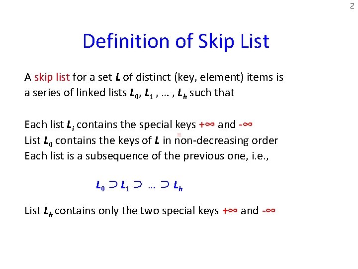
2 Definition of Skip List A skip list for a set L of distinct (key, element) items is a series of linked lists L 0, L 1 , … , Lh such that Each list Li contains the special keys +∞ and -∞ List L 0 contains the keys of L in non-decreasing order Each list is a subsequence of the previous one, i. e. , L 0 ⊃ L 1 ⊃ … ⊃ Lh List Lh contains only the two special keys +∞ and -∞

3 Skip List (Idea due to Pugh ’ 90, CACM paper) Dictionary based on a probabilistic data structure. Allows efficient search, insert, and delete operations. Each element in the dictionary typically stores additional useful information beside its search key. Example: <student id. Transcripts> <date, news> [for University of Iowa] [for Daily Iowan] Probabilistic alternative to a balanced tree.

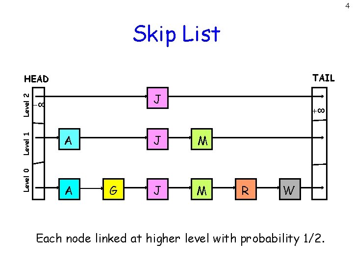
4 Skip List TAIL Level 0 Level 1 Level 2 HEAD J -∞ A A G +∞ J M R W Each node linked at higher level with probability 1/2.

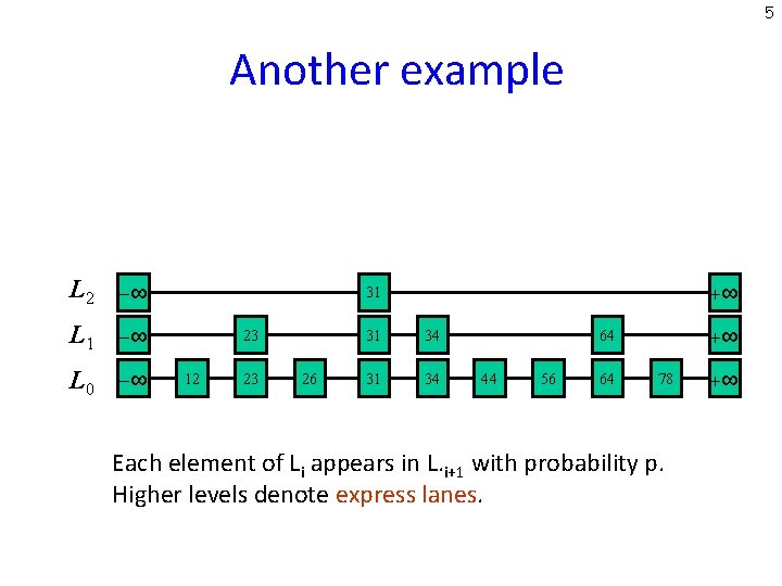
5 Another example L 2 -∞ L 1 -∞ L 0 -∞ +∞ 31 23 12 23 26 31 34 +∞ 64 44 56 64 78 Each element of Li appears in L. i+1 with probability p. Higher levels denote express lanes. +∞

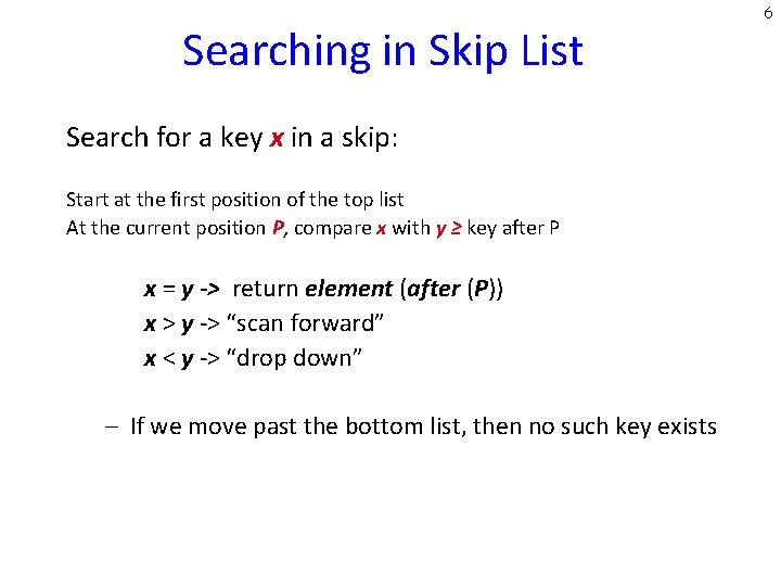
Searching in Skip List Search for a key x in a skip: Start at the first position of the top list At the current position P, compare x with y ≥ key after P x = y -> return element (after (P)) x > y -> “scan forward” x < y -> “drop down” – If we move past the bottom list, then no such key exists 6

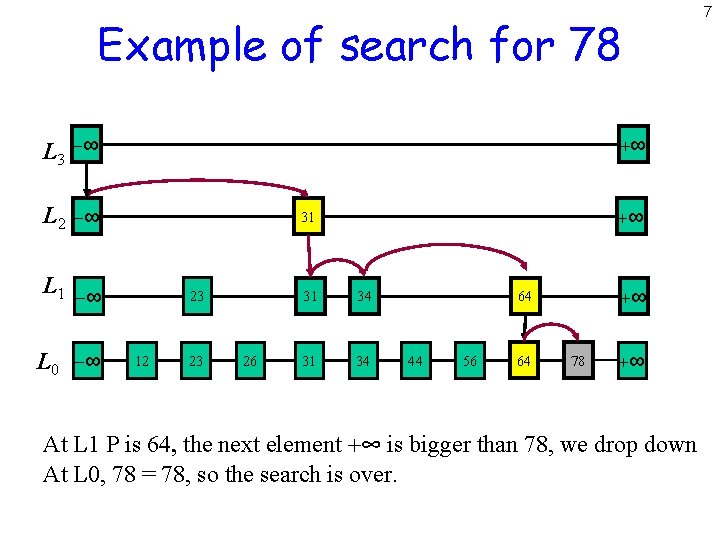
Example of search for 78 L 3 -∞ L 2 -∞ L 1 -∞ L 0 -∞ +∞ +∞ 31 23 12 23 26 31 34 +∞ 64 44 56 64 78 +∞ At L 1 P is 64, the next element +∞ is bigger than 78, we drop down At L 0, 78 = 78, so the search is over. 7

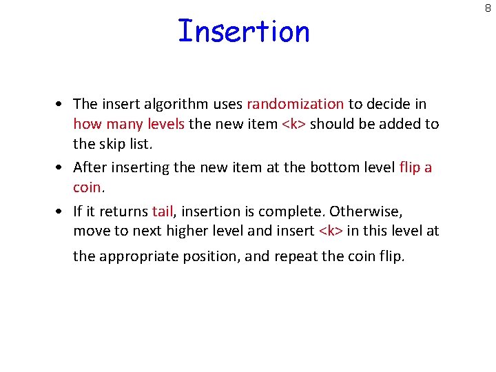
Insertion • The insert algorithm uses randomization to decide in how many levels the new item <k> should be added to the skip list. • After inserting the new item at the bottom level flip a coin. • If it returns tail, insertion is complete. Otherwise, move to next higher level and insert <k> in this level at the appropriate position, and repeat the coin flip. 8

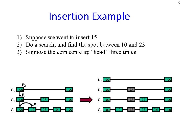
9 Insertion Example 1) Suppose we want to insert 15 2) Do a search, and find the spot between 10 and 23 3) Suppose the coin come up “head” three times p 2 L 2 -∞ p 1 L 1 -∞ L 0 -∞ L 3 -∞ p 0 10 23 23 36 +∞ +∞ L 2 -∞ 15 +∞ L 1 -∞ 15 23 +∞ L 0 -∞ 15 23 10 +∞ +∞ 36 +∞

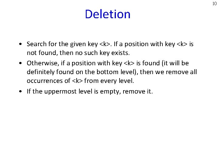
Deletion • Search for the given key <k>. If a position with key <k> is not found, then no such key exists. • Otherwise, if a position with key <k> is found (it will be definitely found on the bottom level), then we remove all occurrences of <k> from every level. • If the uppermost level is empty, remove it. 10

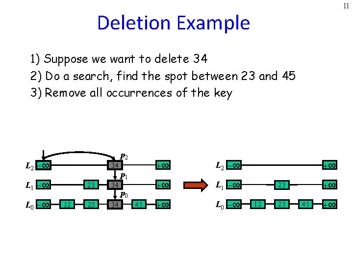
11 Deletion Example 1) Suppose we want to delete 34 2) Do a search, find the spot between 23 and 45 3) Remove all occurrences of the key p 2 L 2 -∞ 34 L 1 -∞ L 0 -∞ 12 23 34 p 1 p 0 45 +∞ L 2 -∞ +∞ L 1 -∞ +∞ L 0 -∞ +∞ +∞ 23 12 23 45 +∞

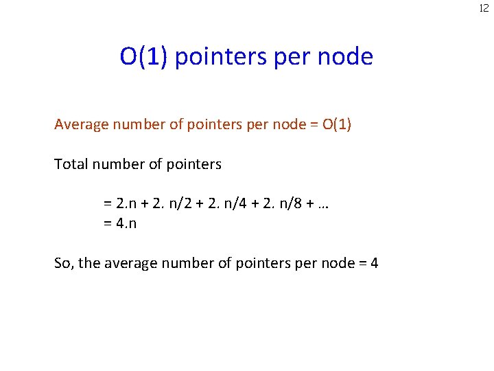
12 O(1) pointers per node Average number of pointers per node = O(1) Total number of pointers = 2. n + 2. n/2 + 2. n/4 + 2. n/8 + … = 4. n So, the average number of pointers per node = 4

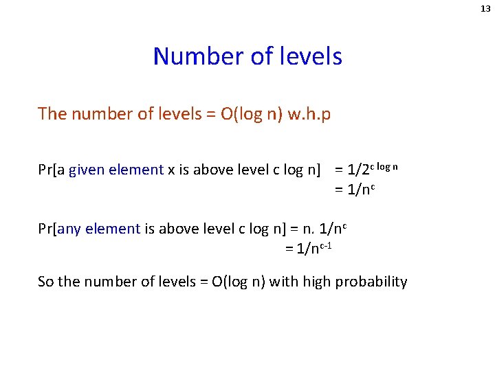
13 Number of levels The number of levels = O(log n) w. h. p Pr[a given element x is above level c log n] = 1/2 c log n = 1/nc Pr[any element is above level c log n] = n. 1/nc = 1/nc-1 So the number of levels = O(log n) with high probability

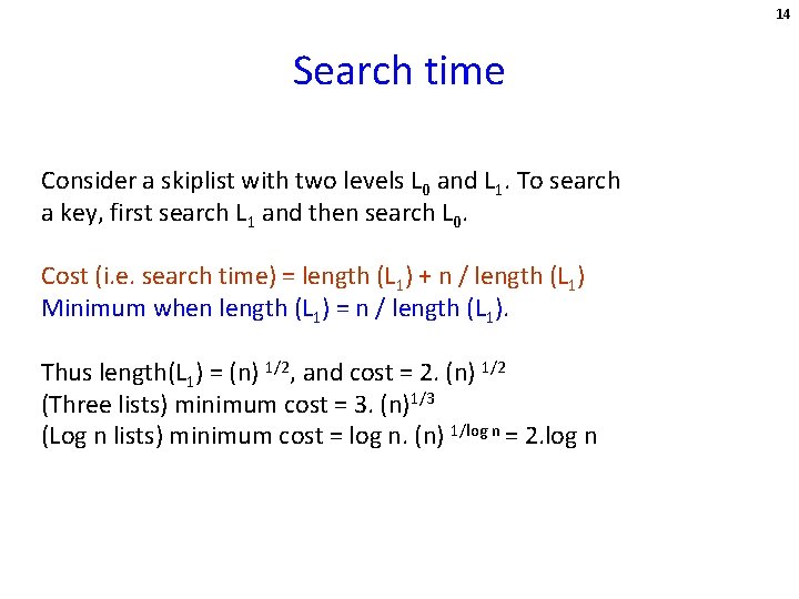
14 Search time Consider a skiplist with two levels L 0 and L 1. To search a key, first search L 1 and then search L 0. Cost (i. e. search time) = length (L 1) + n / length (L 1) Minimum when length (L 1) = n / length (L 1). Thus length(L 1) = (n) 1/2, and cost = 2. (n) 1/2 (Three lists) minimum cost = 3. (n)1/3 (Log n lists) minimum cost = log n. (n) 1/log n = 2. log n

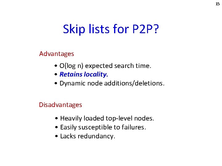
15 Skip lists for P 2 P? Advantages • O(log n) expected search time. • Retains locality. • Dynamic node additions/deletions. Disadvantages • Heavily loaded top-level nodes. • Easily susceptible to failures. • Lacks redundancy.

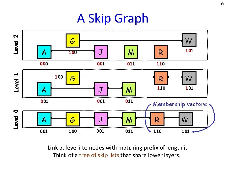
16 Level 2 A Skip Graph A 100 Level 1 000 Level 0 W G 100 J M R 001 011 110 G A J M 001 011 101 R W 110 101 Membership vectors A G J M R W 001 100 001 011 110 101 Link at level i to nodes with matching prefix of length i. Think of a tree of skip lists that share lower layers.

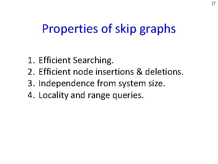
17 Properties of skip graphs 1. 2. 3. 4. Efficient Searching. Efficient node insertions & deletions. Independence from system size. Locality and range queries.

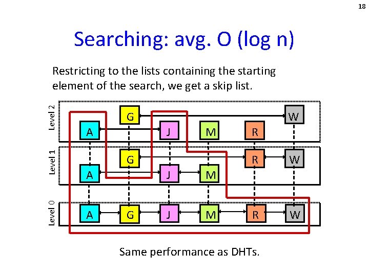
18 Searching: avg. O (log n) Level 0 Level 1 Level 2 Restricting to the lists containing the starting element of the search, we get a skip list. G A W J M G A A G J M R R W Same performance as DHTs.

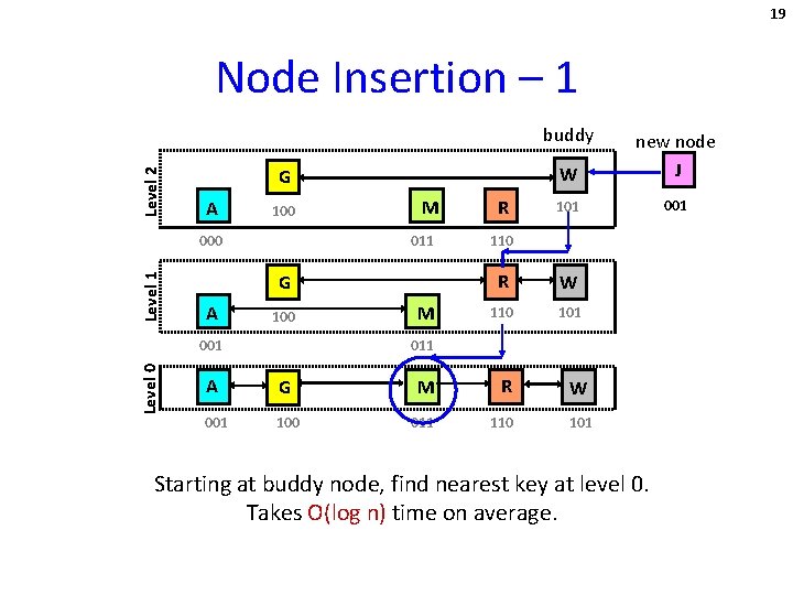
19 Node Insertion – 1 Level 2 buddy G A 100 Level 1 000 011 G A 100 001 Level 0 M M R W new node J 101 001 110 R W 110 101 011 A G M R 001 100 011 110 W 101 Starting at buddy node, find nearest key at level 0. Takes O(log n) time on average.

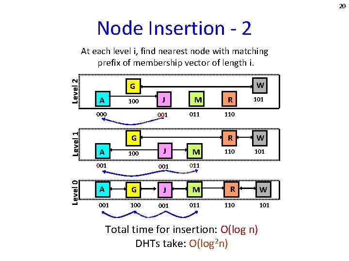
20 Node Insertion - 2 Level 2 At each level i, find nearest node with matching prefix of membership vector of length i. A 100 Level 1 000 J 001 M 011 G A 100 001 Level 0 W G J M 001 011 R 101 110 R W 110 101 A G J M R 001 100 001 011 110 Total time for insertion: O(log n) DHTs take: O(log 2 n) W 101

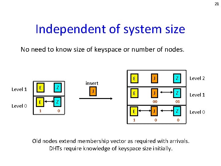
21 Independent of system size No need to know size of keyspace or number of nodes. Level 1 Level 0 E Z 1 0 insert J E J Z Level 2 E J Z Level 1 00 01 J Z E 1 0 0 Old nodes extend membership vector as required with arrivals. DHTs require knowledge of keyspace size initially. Level 0

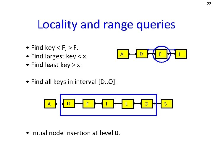
22 Locality and range queries • Find key < F, > F. • Find largest key < x. • Find least key > x. D A F I • Find all keys in interval [D. . O]. A D F I • Initial node insertion at level 0. L O S

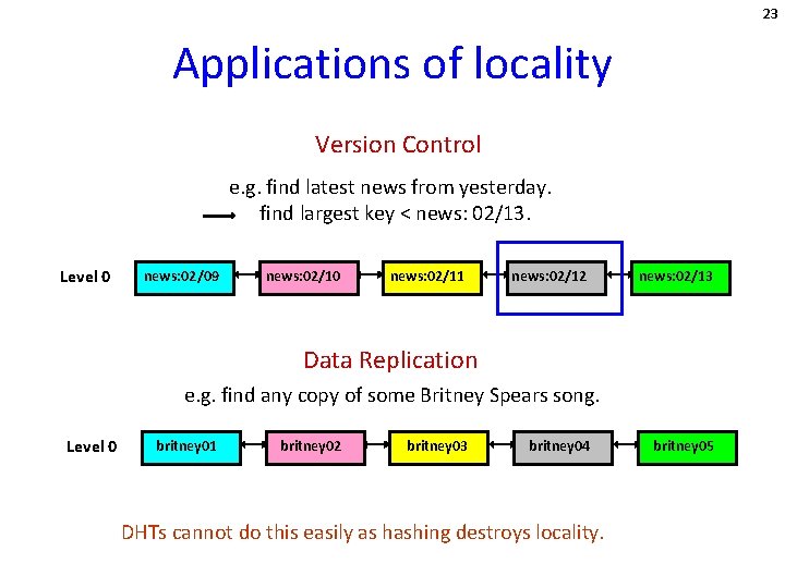
23 Applications of locality Version Control e. g. find latest news from yesterday. find largest key < news: 02/13. Level 0 news: 02/09 news: 02/10 news: 02/11 news: 02/12 news: 02/13 Data Replication e. g. find any copy of some Britney Spears song. Level 0 britney 01 britney 02 britney 03 britney 04 DHTs cannot do this easily as hashing destroys locality. britney 05

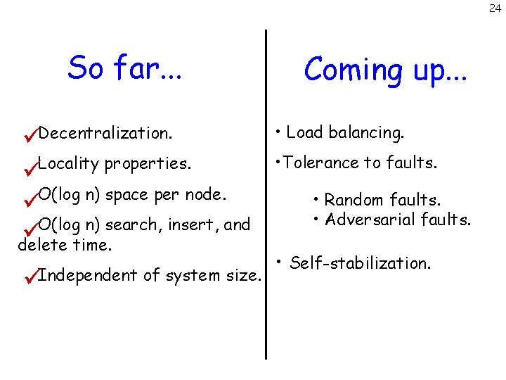
24 So far. . . Decentralization. Locality properties. O(log n) space per node. O(log n) search, insert, and delete time. Independent of system size. Coming up. . . • Load balancing. • Tolerance to faults. • Random faults. • Adversarial faults. • Self-stabilization.

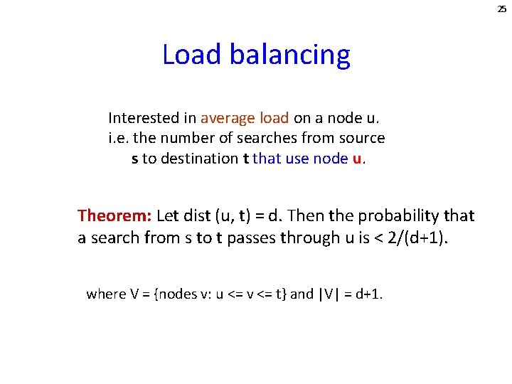
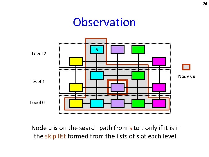
25 Load balancing Interested in average load on a node u. i. e. the number of searches from source s to destination t that use node u. Theorem: Let dist (u, t) = d. Then the probability that a search from s to t passes through u is < 2/(d+1). where V = {nodes v: u <= v <= t} and |V| = d+1.

26 Observation Level 2 Level 1 s Nodes u Level 0 Node u is on the search path from s to t only if it is in the skip list formed from the lists of s at each level.

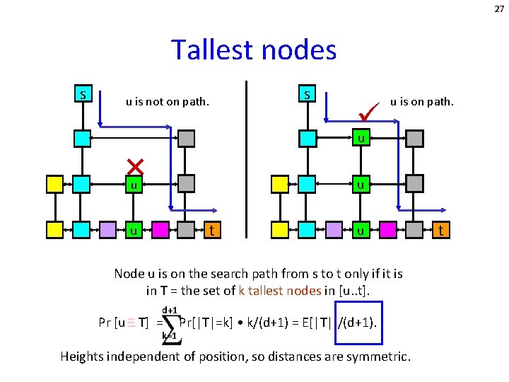
27 Tallest nodes s s u is not on path. u is on path. u u u t u u Node u is on the search path from s to t only if it is in T = the set of k tallest nodes in [u. . t]. d+1 Pr [u T] = k=1 Pr[|T|=k] • k/(d+1) = E[|T|]/(d+1). Heights independent of position, so distances are symmetric. t

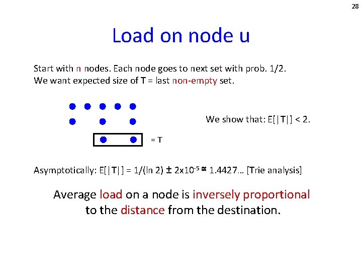
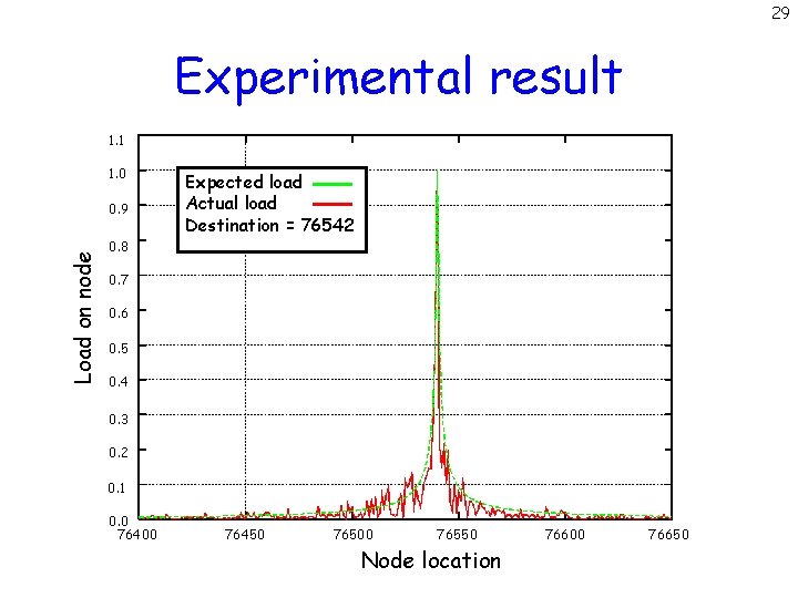
28 Load on node u Start with n nodes. Each node goes to next set with prob. 1/2. We want expected size of T = last non-empty set. We show that: E[|T|] < 2. =T Asymptotically: E[|T|] = 1/(ln 2) ± 2 x 10 -5 ≃ 1. 4427… [Trie analysis] Average load on a node is inversely proportional to the distance from the destination.

29 Experimental result 1. 1 1. 0 Load on node 0. 9 Expected load Actual load Destination = 76542 0. 8 0. 7 0. 6 0. 5 0. 4 0. 3 0. 2 0. 1 0. 0 76400 76450 76500 76550 Node location 76600 76650

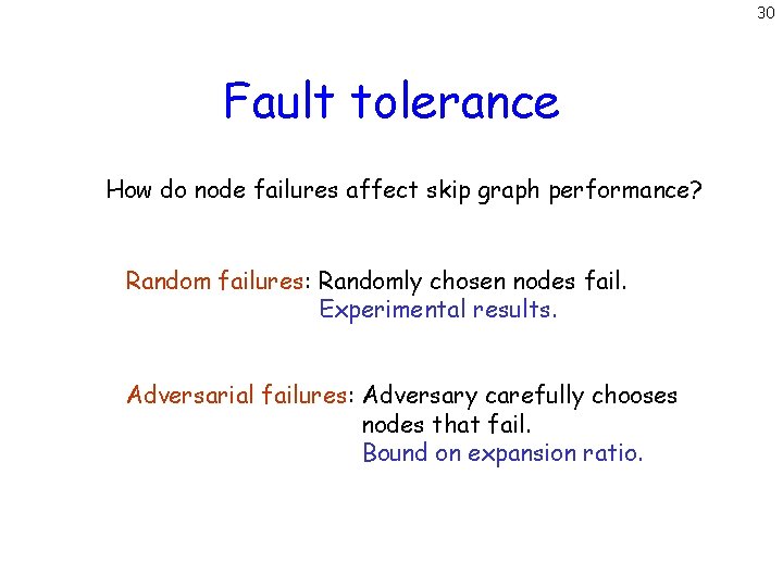
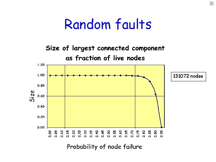
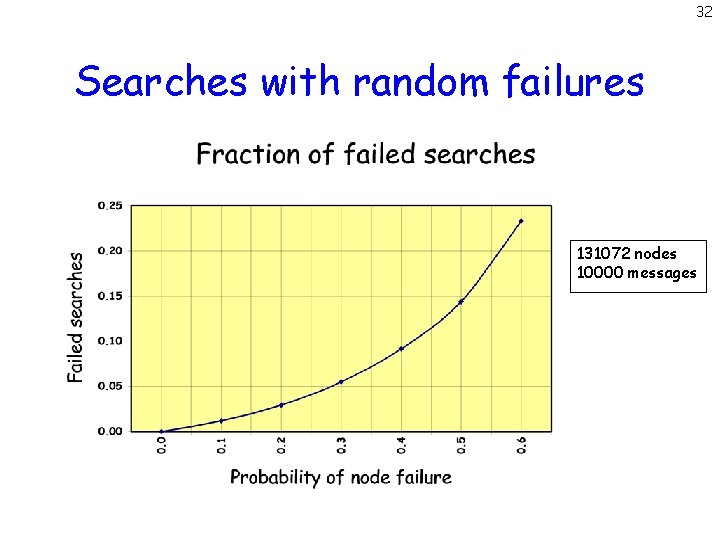
30 Fault tolerance How do node failures affect skip graph performance? Random failures: Randomly chosen nodes fail. Experimental results. Adversarial failures: Adversary carefully chooses nodes that fail. Bound on expansion ratio.

31 Random faults 131072 nodes

32 Searches with random failures 131072 nodes 10000 messages

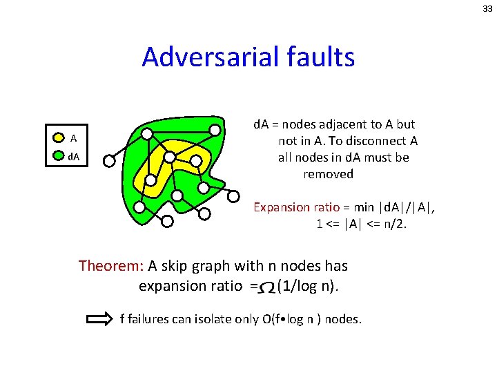
33 Adversarial faults A d. A = nodes adjacent to A but not in A. To disconnect A all nodes in d. A must be removed Expansion ratio = min |d. A|/|A|, 1 <= |A| <= n/2. Theorem: A skip graph with n nodes has expansion ratio = (1/log n). f failures can isolate only O(f • log n ) nodes.

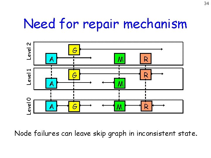
34 Level 0 Level 1 Level 2 Need for repair mechanism A A A G G G J M J M R W R W Node failures can leave skip graph in inconsistent state.

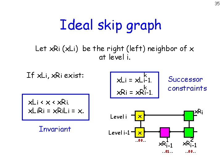
35 Ideal skip graph Let x. Ri (x. Li) be the right (left) neighbor of x at level i. If x. Li, x. Ri exist: x. Li < x. Ri. x. Li. Ri = x. Ri. Li = x. Invariant k x. Li = x. Li-1. k x. Ri = x. Ri-1. Level i x Level i-1 x. . 00. . Successor constraints x. Ri 1 x. R i-1 . . 01. . 2 x. R i-1. . 00. .

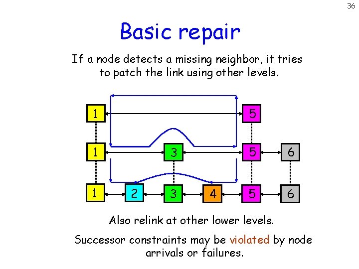
36 Basic repair If a node detects a missing neighbor, it tries to patch the link using other levels. 5 1 1 1 3 2 3 4 5 6 Also relink at other lower levels. Successor constraints may be violated by node arrivals or failures.

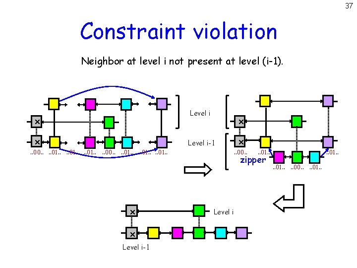
37 Constraint violation Neighbor at level i not present at level (i-1). Level i x x. . 00. . . . 01. . x x Level i-1 . . 00. . 01. . zipper Level i . . 01. . . . 00. . 01. .

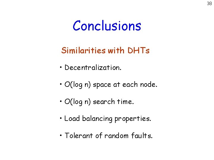
38 Conclusions Similarities with DHTs • Decentralization. • O(log n) space at each node. • O(log n) search time. • Load balancing properties. • Tolerant of random faults.

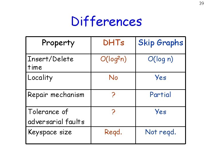
39 Differences Property DHTs Skip Graphs O(log 2 n) O(log n) No Yes Repair mechanism ? Partial Tolerance of adversarial faults Keyspace size ? Yes Reqd. Not reqd. Insert/Delete time Locality

40 Open Problems • Design efficient repair mechanism. • Incorporate geographical proximity. • Study multi-dimensional skip graphs. • Evaluate performance in practice. • Study effect of byzantine failures. ?