SKIP GRAPHS Slides adapted from the original slides

SKIP GRAPHS Slides adapted from the original slides by James Aspnes Gauri Shah

2 Skip List [Pugh ’ 90] Data structure based on a linked list. HEAD J Level 2 Level 1 Level 0 TAIL A A G J M R W Each node linked at higher level with probability 1/2.

3 Skip List [Pugh ’ 90] Probabilistic alternative to balanced trees. L 0 = linked list of ALL nodes ordered by key. Each element of Li appears in L. i+1 with prob p. Higher levels denote express lanes. We will only consider p=1/2

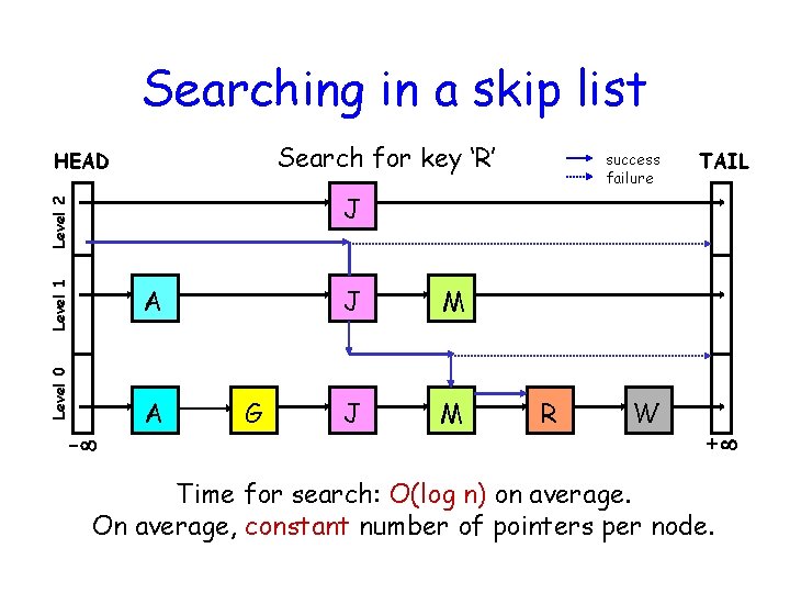
Searching in a skip list Search for key ‘R’ HEAD success failure TAIL Level 1 Level 2 J Level 0 A - A G J M R W + Time for search: O(log n) on average. On average, constant number of pointers per node.

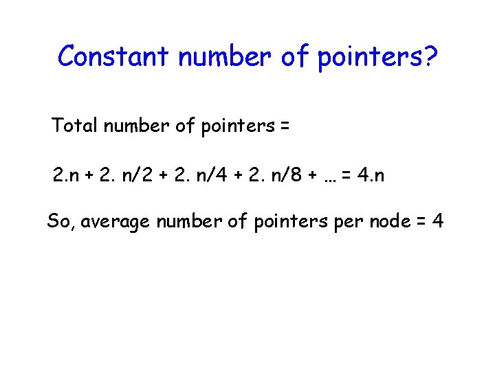
Constant number of pointers? Total number of pointers = 2. n + 2. n/2 + 2. n/4 + 2. n/8 + … = 4. n So, average number of pointers per node = 4

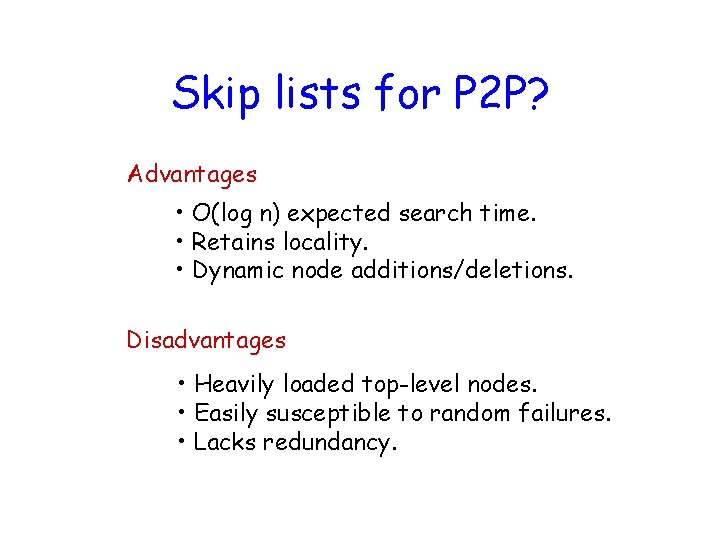
Skip lists for P 2 P? Advantages • O(log n) expected search time. • Retains locality. • Dynamic node additions/deletions. Disadvantages • Heavily loaded top-level nodes. • Easily susceptible to random failures. • Lacks redundancy.

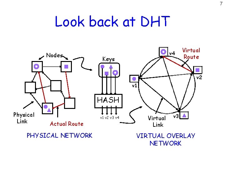
7 Look back at DHT Nodes v 4 Keys Virtual Route v 2 v 1 HASH Physical Link Actual Route PHYSICAL NETWORK v 1 v 2 v 3 v 4 Virtual Link v 3 VIRTUAL OVERLAY NETWORK

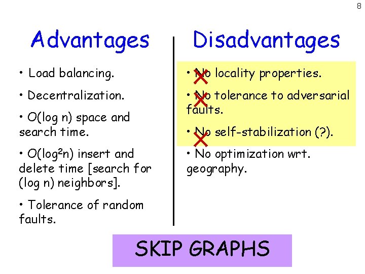
8 Advantages Disadvantages • Load balancing. • No locality properties. • Decentralization. • No tolerance to adversarial faults. • O(log n) space and search time. • No self-stabilization (? ). • O(log 2 n) insert and delete time [search for (log n) neighbors]. • No optimization wrt. geography. • Tolerance of random faults. SKIP GRAPHS

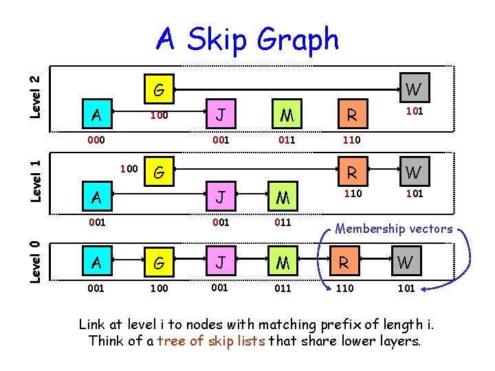
Level 2 A Skip Graph A 100 Level 1 000 Level 0 W G 100 J M R 001 011 110 G A J M 001 011 101 R W 110 101 Membership vectors A G J M R W 001 100 001 011 110 101 Link at level i to nodes with matching prefix of length i. Think of a tree of skip lists that share lower layers.

Properties of skip graphs 1. Efficient Searching. 2. Eficient node insertions & deletions. 3. Independence from system size. 4. Locality and range queries.

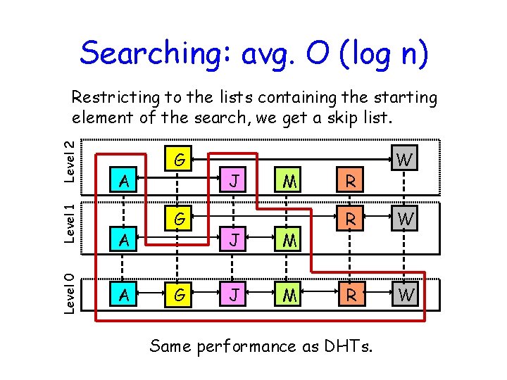
Searching: avg. O (log n) Level 0 Level 1 Level 2 Restricting to the lists containing the starting element of the search, we get a skip list. A A A G G G J M J M R W R W Same performance as DHTs.

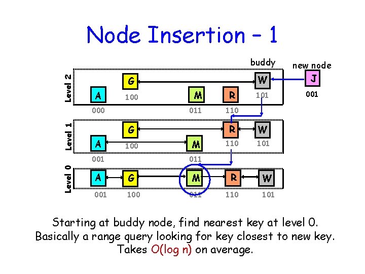
Node Insertion – 1 Level 2 buddy G A 100 Level 1 000 011 A 100 R 101 001 110 R W 110 101 M R W 011 110 101 G 001 Level 0 M W new node J M 011 A G 001 100 Starting at buddy node, find nearest key at level 0. Basically a range query looking for key closest to new key. Takes O(log n) on average.

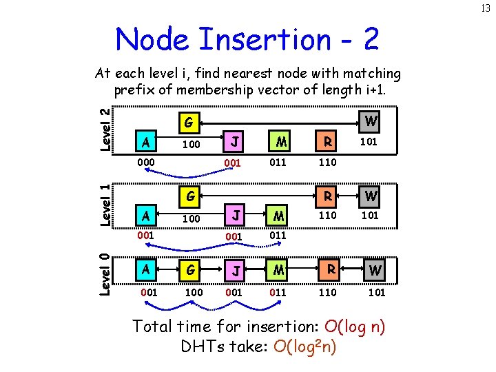
13 Node Insertion - 2 Level 2 At each level i, find nearest node with matching prefix of membership vector of length i+1. A 100 Level 1 000 J M 001 011 G A 100 001 Level 0 W G A G 001 100 R 101 110 R W 110 101 W J M 001 011 J M R 001 011 110 101 Total time for insertion: O(log n) DHTs take: O(log 2 n)

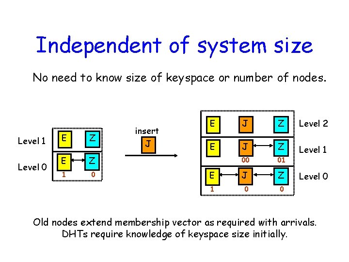
Independent of system size No need to know size of keyspace or number of nodes. Level 1 Level 0 E Z 1 0 insert J E J Z Level 2 E J Z 00 01 Level 1 E J Z 1 0 0 Level 0 Old nodes extend membership vector as required with arrivals. DHTs require knowledge of keyspace size initially.

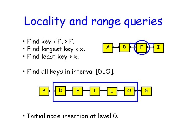
Locality and range queries • Find key < F, > F. • Find largest key < x. • Find least key > x. D A F I • Find all keys in interval [D. . O]. A D F I L • Initial node insertion at level 0. O S

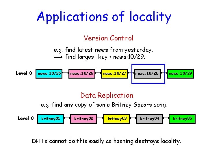
Applications of locality Version Control e. g. find latest news from yesterday. find largest key < news: 10/29. Level 0 news: 10/25 news: 10/26 news: 10/27 news: 10/28 news: 10/29 Data Replication e. g. find any copy of some Britney Spears song. Level 0 britney 01 britney 02 britney 03 britney 04 britney 05 DHTs cannot do this easily as hashing destroys locality.

17 So far. . . Decentralization. Locality properties. O(log n) space per node. O(log n) search, insert, and delete time. Independent of system size. Coming up. . . • Load balancing. • Tolerance to faults. • Random faults. • Adversarial faults. • Self-stabilization.

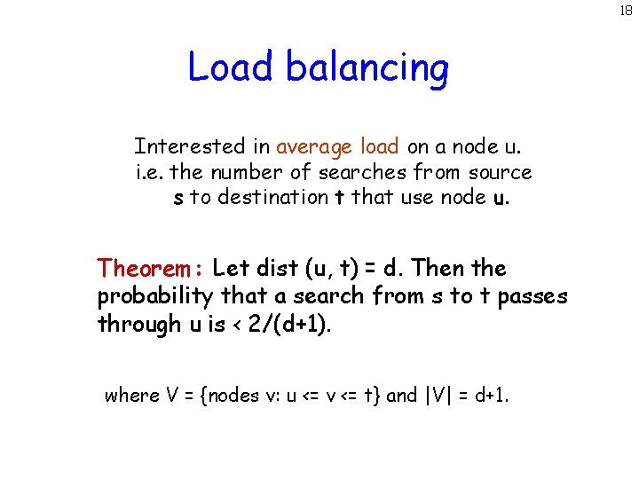
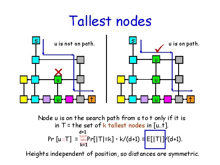
18 Load balancing Interested in average load on a node u. i. e. the number of searches from source s to destination t that use node u. Theorem: Let dist (u, t) = d. Then the probability that a search from s to t passes through u is < 2/(d+1). where V = {nodes v: u <= v <= t} and |V| = d+1.

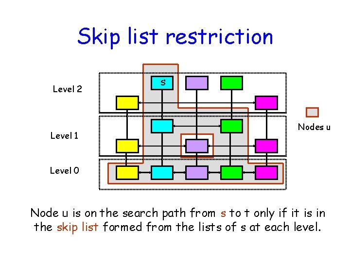
Skip list restriction Level 2 Level 1 s Nodes u Level 0 Node u is on the search path from s to t only if it is in the skip list formed from the lists of s at each level.

Tallest nodes s u is not on path. s u is on path. u u u t Node u is on the search path from s to t only if it is in T = the set of k tallest nodes in [u. . t]. Pr [u T] = d+1 Pr[|T|=k] • k/(d+1) = E[|T|]/(d+1). k=1 Heights independent of position, so distances are symmetric.