SKIP GRAPHS continued Some slides adapted from the

SKIP GRAPHS (continued) Some slides adapted from the original slides by James Aspnes Gauri Shah

2 So far. . . Decentralization. Locality properties. O(log n) neighbors per node. O(log n) search, insert, and delete time. Independent of system size. Coming up. . . • Load balancing. • Tolerance to faults. • Random faults. • Adversarial faults. • Self-stabilization.

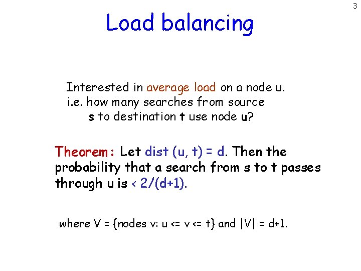
Load balancing Interested in average load on a node u. i. e. how many searches from source s to destination t use node u? Theorem: Let dist (u, t) = d. Then the probability that a search from s to t passes through u is < 2/(d+1). where V = {nodes v: u <= v <= t} and |V| = d+1. 3

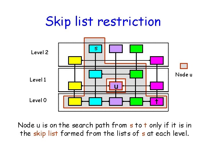
Skip list restriction Level 2 Level 1 Level 0 s Node u u t Node u is on the search path from s to t only if it is in the skip list formed from the lists of s at each level.

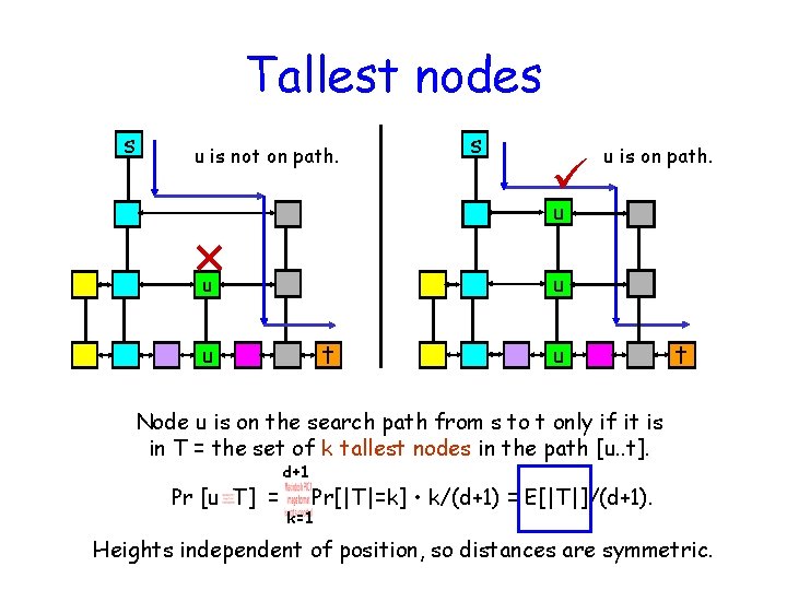
Tallest nodes s u is not on path. s u is on path. u u u t Node u is on the search path from s to t only if it is in T = the set of k tallest nodes in the path [u. . t]. Pr [u T] = d+1 Pr[|T|=k] • k/(d+1) = E[|T|]/(d+1). k=1 Heights independent of position, so distances are symmetric.

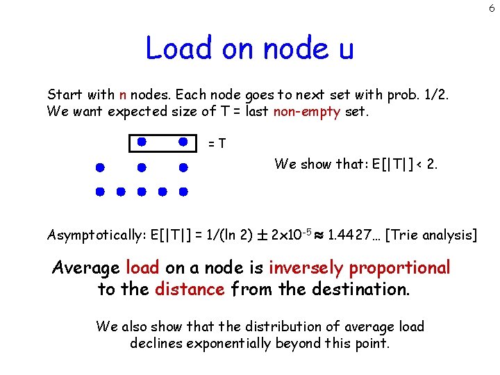
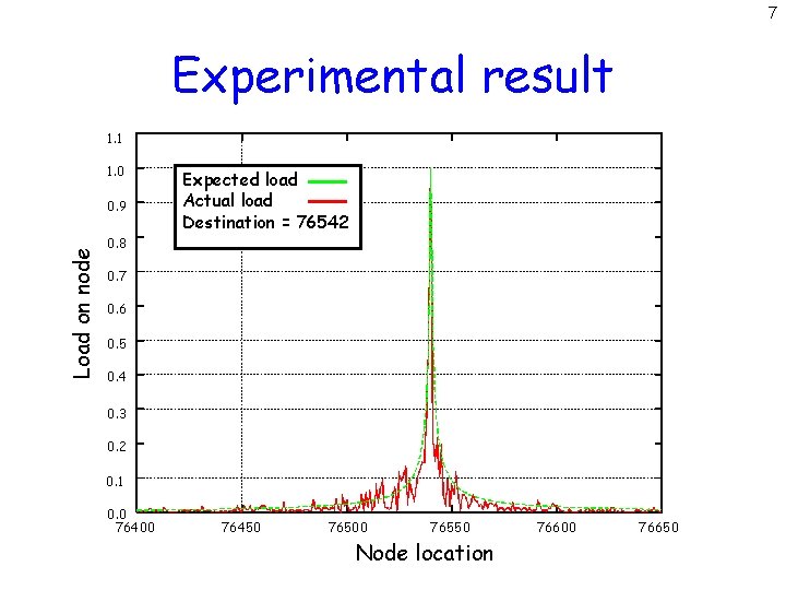
6 Load on node u Start with n nodes. Each node goes to next set with prob. 1/2. We want expected size of T = last non-empty set. =T We show that: E[|T|] < 2. Asymptotically: E[|T|] = 1/(ln 2) 2 x 10 -5 1. 4427… [Trie analysis] Average load on a node is inversely proportional to the distance from the destination. We also show that the distribution of average load declines exponentially beyond this point.

7 Experimental result 1. 1 1. 0 Load on node 0. 9 Expected load Actual load Destination = 76542 0. 8 0. 7 0. 6 0. 5 0. 4 0. 3 0. 2 0. 1 0. 0 76400 76450 76500 76550 Node location 76600 76650

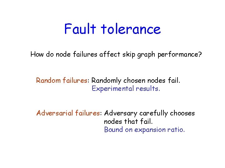
Fault tolerance How do node failures affect skip graph performance? Random failures: Randomly chosen nodes fail. Experimental results. Adversarial failures: Adversary carefully chooses nodes that fail. Bound on expansion ratio.

Random faults 131072 nodes

Searches with random failures 131072 nodes 10000 messages

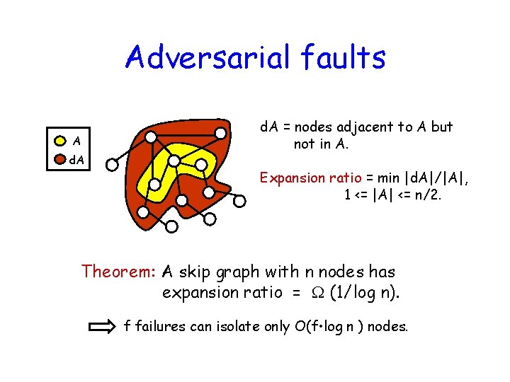
Adversarial faults A d. A = nodes adjacent to A but not in A. Expansion ratio = min |d. A|/|A|, 1 <= |A| <= n/2. Theorem: A skip graph with n nodes has expansion ratio = (1/log n). f failures can isolate only O(f • log n ) nodes.

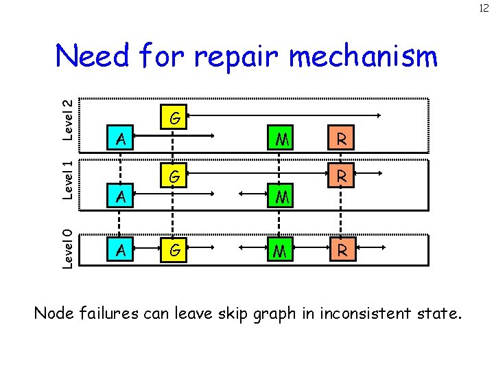
12 Level 0 Level 1 Level 2 Need for repair mechanism A A A G G G J M J M R W R W Node failures can leave skip graph in inconsistent state.

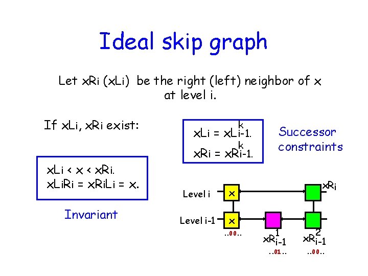
Ideal skip graph Let x. Ri (x. Li) be the right (left) neighbor of x at level i. If x. Li, x. Ri exist: x. Li < x. Ri. x. Li. Ri = x. Ri. Li = x. Invariant k x. Li = x. Li-1. k x. Ri = x. Ri-1. Level i x Level i-1 x. . 00. . Successor constraints x. Ri 1 x. R i-1 . . 01. . 2 x. R i-1. . 00. .

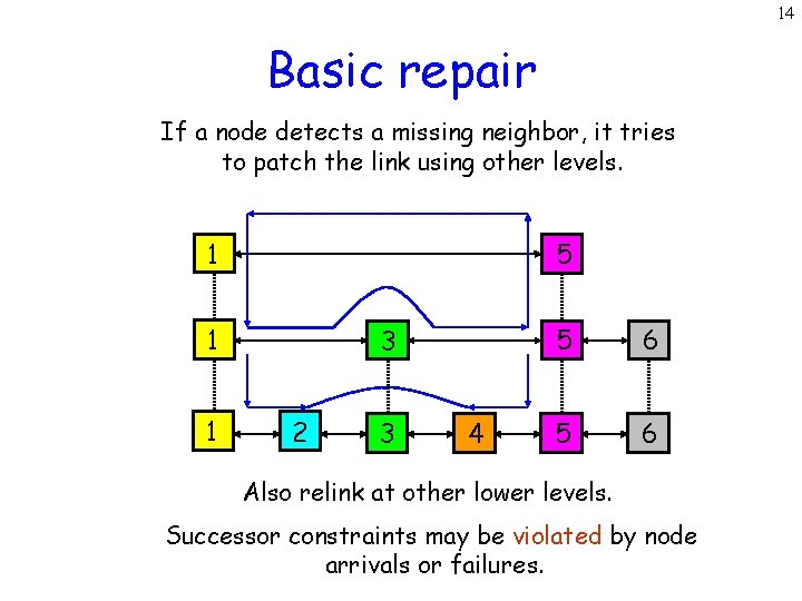
14 Basic repair If a node detects a missing neighbor, it tries to patch the link using other levels. 5 1 1 1 3 2 3 4 5 6 Also relink at other lower levels. Successor constraints may be violated by node arrivals or failures.

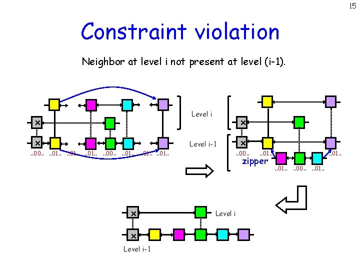
15 Constraint violation Neighbor at level i not present at level (i-1). Level i x x. . 00. . . . 01. . x x Level i-1 . . 00. . 01. . zipper Level i . . 01. . . . 00. . 01. .

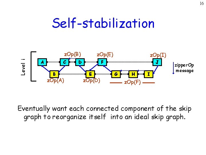
16 Self-stabilization Level i z. Op(B) A C B z. Op(A) z. Op(E) D z. Op(I) F E z. Op(D) J G H I zipper. Op message z. Op(F) Eventually want each connected component of the skip graph to reorganize itself into an ideal skip graph.

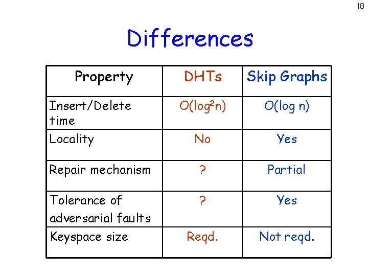
Conclusions Similarities with DHTs • Decentralization. • O(log n) space at each node. • O(log n) search time. • Load balancing properties. • Tolerant of random faults.

18 Differences Property DHTs Skip Graphs O(log 2 n) O(log n) No Yes Repair mechanism ? Partial Tolerance of adversarial faults Keyspace size ? Yes Reqd. Not reqd. Insert/Delete time Locality

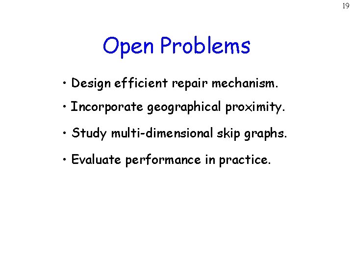
19 Open Problems • Design efficient repair mechanism. • Incorporate geographical proximity. • Study multi-dimensional skip graphs. • Evaluate performance in practice.