SKEW IN PARALLEL QUERY PROCESSING Paraschos Koutris Paul

SKEW IN PARALLEL QUERY PROCESSING Paraschos Koutris Paul Beame Dan Suciu University of Washington PODS 2014

MOTIVATION • Understand the complexity of parallel query processing on big data – on shared-nothing architectures (e. g. Map. Reduce) – even in the presence of data skew • Dominating parameters of computation: – Communication cost – Number of communication rounds 2

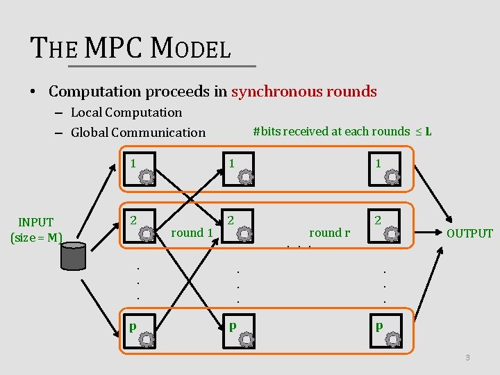
THE MPC MODEL • Computation proceeds in synchronous rounds – Local Computation – Global Communication INPUT (size = M) #bits received at each rounds ≤ L 1 1 1 2 2 2 round 1. . . p round r. . p OUTPUT p 3

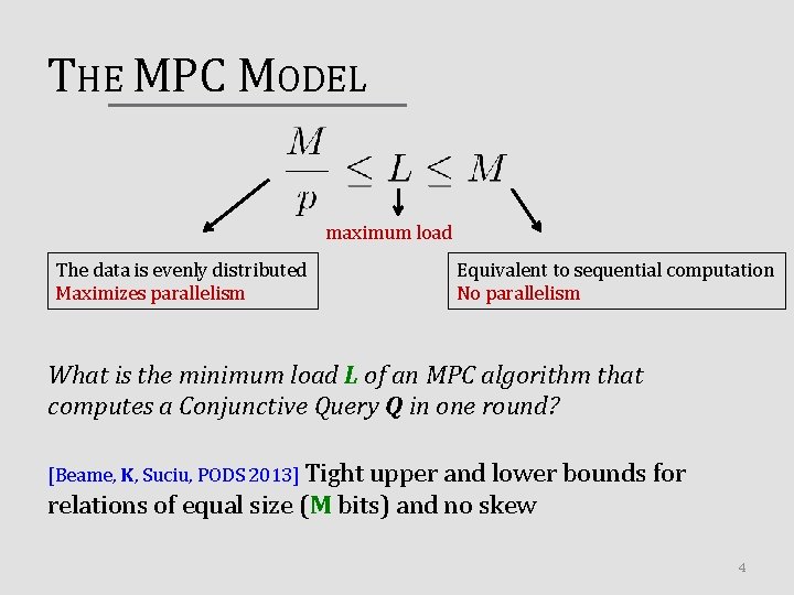
THE MPC MODEL maximum load The data is evenly distributed Maximizes parallelism Equivalent to sequential computation No parallelism What is the minimum load L of an MPC algorithm that computes a Conjunctive Query Q in one round? [Beame, K, Suciu, PODS 2013] Tight upper and lower bounds for relations of equal size (M bits) and no skew 4

RESULTS Computing a Conjunctive Query Q in the MPC model in one round for relations with different sizes and skew • Matching upper and lower bounds for any skew-free input database and different relation sizes • Almost matching upper and lower bounds in the presence of skew – Matching bounds in the case of simple joins 5

CONJUNCTIVE QUERIES • Full Conjuctive Queries w/o self-joins: – Q(x, y, z) = R(x, y), S(y, z), T(z, x) [the triangle query] • The hypergraph of the query Q: – Variables as vertices – Atoms as hyperedges x T R y z S 6

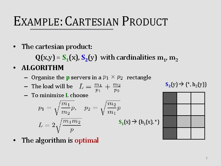
EXAMPLE: CARTESIAN PRODUCT • The cartesian product: Q(x, y) = S 1(x), S 2(y) with cardinalities m 1, m 2 • ALGORITHM – Organize the p servers in a – The load will be – To minimize L choose rectangle S 2(y) (*, h 2(y)) S 1(x) (h 1(x), *) • The algorithm is optimal 7

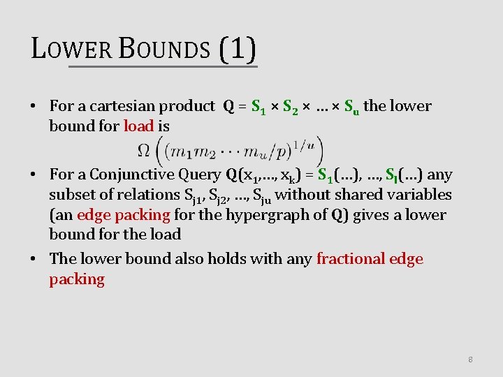
LOWER BOUNDS (1) • For a cartesian product Q = S 1 × S 2 × … × Su the lower bound for load is • For a Conjunctive Query Q(x 1, …, xk) = S 1(…), …, Sl(…) any subset of relations Sj 1, Sj 2, …, Sju without shared variables (an edge packing for the hypergraph of Q) gives a lower bound for the load • The lower bound also holds with any fractional edge packing 8

LOWER BOUNDS (2) Theorem For a Conjunctive Query Q, where relation Sj has size Mj (in bits), any MPC algorithm that computes Q in one round with maximum load L must satisfy for some constant c and for any fractional edge packing u: Proof techniques: • Using entropy to bound knowledge • Friedgut’s inequality to bound the maximum size of a query 9

HYPERCUBE ALGORITHM • Q(x 1, …, xk) = S 1(…), …, Sl(…) • For each variable xi define the share to be an integer pi such that: p = p 1 ×. . × pk • Assign each of the p servers to a point on the kdimensional hypercube: [p] = [p 1] × … × [pk] • Hash each tuple to the appropriate subcube e. g. S 3 (x 3, x 4) (* , *, h 3(x 3), h 4(x 4), *, …) 10

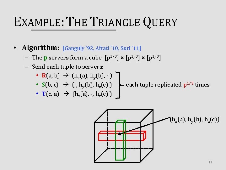
EXAMPLE: THE TRIANGLE QUERY • Algorithm: [Ganguly ’ 92, Afrati ’ 10, Suri ’ 11] – The p servers form a cube: [p 1/3] × [p 1/3] – Send each tuple to servers: • R(a, b) (hx(a), hy(b), - ) • S(b, c) (-, hy(b), hz(c) ) each tuple replicated p 1/3 times • T(c, a) (hx(a), -, hz(c) ) (hx(a), hy(b), hz(c)) 11

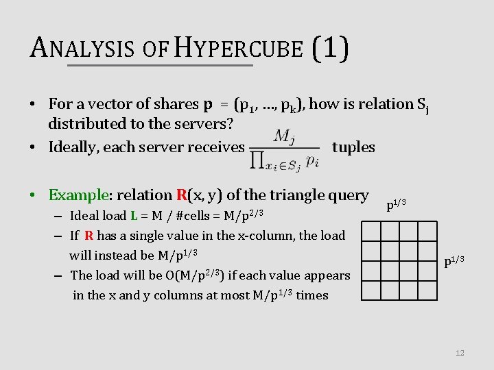
ANALYSIS OF HYPERCUBE (1) • For a vector of shares p = (p 1, …, pk), how is relation Sj distributed to the servers? • Ideally, each server receives tuples • Example: relation R(x, y) of the triangle query – Ideal load L = M / #cells = M/p 2/3 – If R has a single value in the x-column, the load will instead be M/p 1/3 – The load will be O(M/p 2/3) if each value appears in the x and y columns at most M/p 1/3 times p 1/3 12

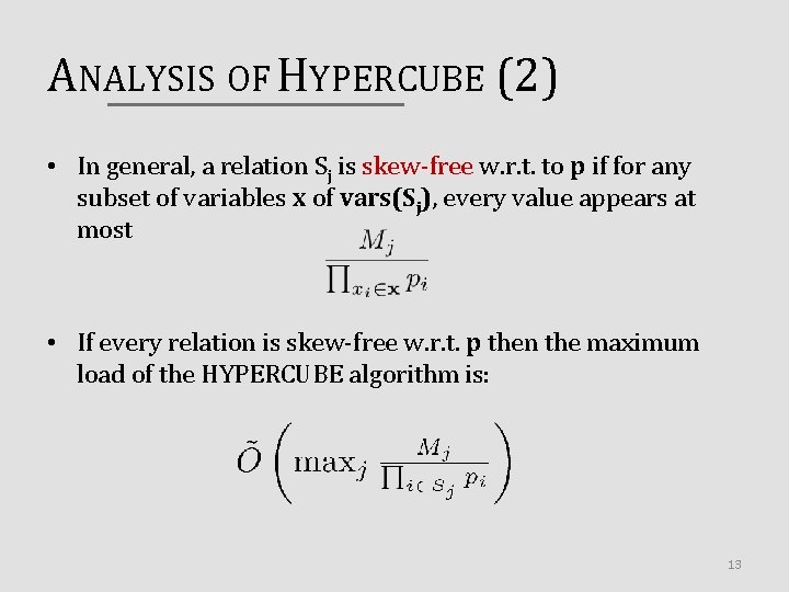
ANALYSIS OF HYPERCUBE (2) • In general, a relation Sj is skew-free w. r. t. to p if for any subset of variables x of vars(Sj), every value appears at most • If every relation is skew-free w. r. t. p then the maximum load of the HYPERCUBE algorithm is: 13

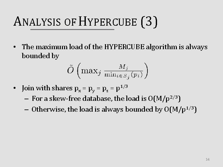
ANALYSIS OF HYPERCUBE (3) • The maximum load of the HYPERCUBE algorithm is always bounded by • Join with shares px = py = pz = p 1/3 – For a skew-free database, the load is O(M/p 2/3) – Otherwise, the load is always bounded by O(M/p 1/3) 14

COMPUTING THE SHARES • The optimal shares Linear Program (LP) are computed by solving a 15

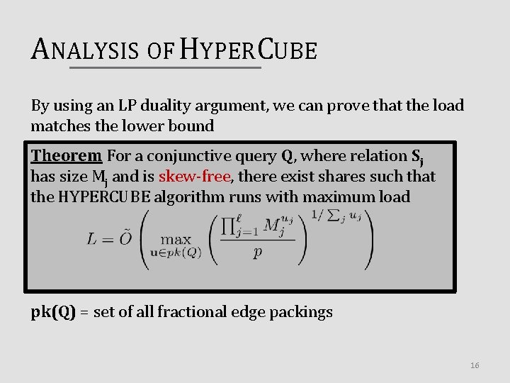
ANALYSIS OF HYPERCUBE By using an LP duality argument, we can prove that the load matches the lower bound Theorem For a conjunctive query Q, where relation Sj has size Mj and is skew-free, there exist shares such that the HYPERCUBE algorithm runs with maximum load pk(Q) = set of all fractional edge packings 16

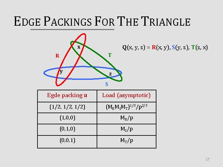
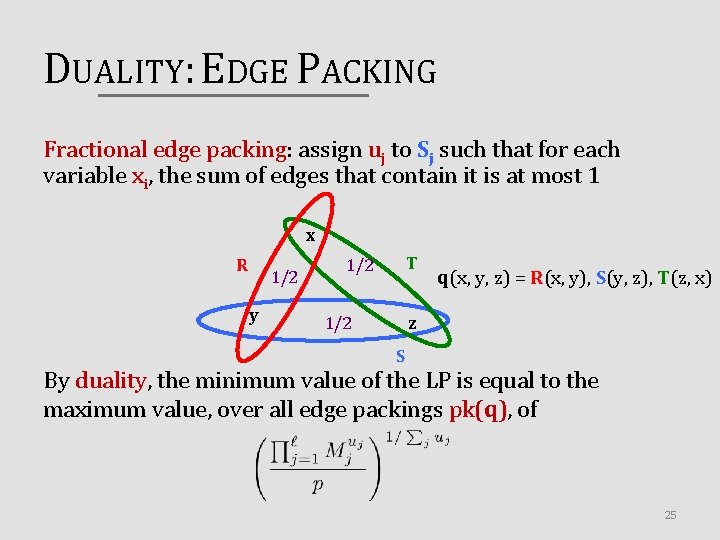
EDGE PACKINGS FOR THE TRIANGLE x Q(x, y, z) = R(x, y), S(y, z), T(z, x) T R y z S Egde packing u Load (asymptotic) (1/2, 1/2) (MRMSMT)1/3/p 2/3 (1, 0, 0) MR/p (0, 1, 0) MS/p (0, 0, 1) MT/p 17

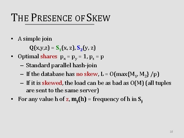
THE PRESENCE OF SKEW • A simple join Q(x, y, z) = S 1(x, z), S 2(y, z) • Optimal shares px = py = 1, pz = p – Standard parallel hash-join – If the database has no skew, L = O(max{M 1, M 2} /p) – If it is skewed, the load can be as bad as O(M) (all tuples are sent to the same server) • For any value h of z, mj(h) = frequency of h in Sj 18

SKEW-AWARE JOIN (1) Q(x, y, z) = S 1(x, z), S 2(y, z) • Idea: identify the heavy hitters and treat them differently • h is a heavy hitter in Sj if mj(h) > Mj/p • h is light otherwise CASE 1 (LIGHT) • For all light values h, run the Hyper. Cube algorithm (hashjoin on z) on all p servers 19

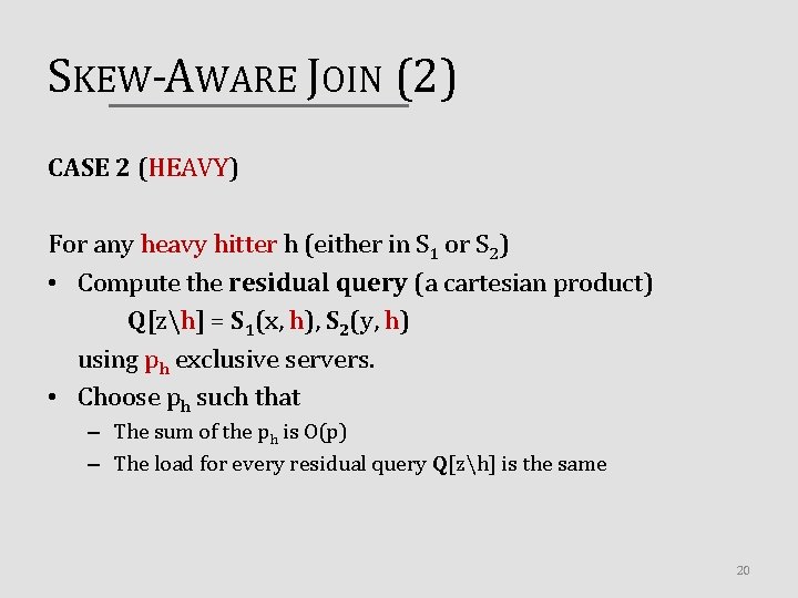
SKEW-AWARE JOIN (2) CASE 2 (HEAVY) For any heavy hitter h (either in S 1 or S 2) • Compute the residual query (a cartesian product) Q[zh] = S 1(x, h), S 2(y, h) using ph exclusive servers. • Choose ph such that – The sum of the ph is O(p) – The load for every residual query Q[zh] is the same 20

SKEW: SIMPLE JOIN Theorem Any MPC algorithm that computes the join query in one round must satisfy: The skew-aware join achieves the above optimal load 21

SKEW IN CONJUNCTIVE QUERIES • For any conjunctive query Q, our algorithm computes the light values using HYPERCUBE – Since there is no skew, this part is optimal • For the heavy hitters, it considers the residual queries and assigns appropriately an exclusive number of servers – The values of the heavy hitters and their frequency must be known to the algorithm 22

CONCLUSION Summary • Upper and lower bounds for computing Conjunctive Queries in the MPC model in the presence of skew Open Problems • What is the load L when we consider more rounds? • How do other classes of queries behave? 23

Thank you ! 24

DUALITY: EDGE PACKING Fractional edge packing: assign uj to Sj such that for each variable xi, the sum of edges that contain it is at most 1 x R 1/2 y T 1/2 q(x, y, z) = R(x, y), S(y, z), T(z, x) z 1/2 S By duality, the minimum value of the LP is equal to the maximum value, over all edge packings pk(q), of 25