Sketching Graphs Horizontal Vertical Oblique Determining intervals of

Sketching Graphs

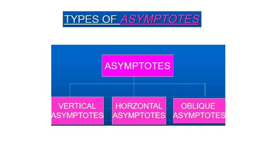
Horizontal Vertical Oblique

Determining intervals of monotonocity

Definitions of Increasing and Decreasing Functions

c inc de inc A function is increasing when its graph rises as it goes from left to right. A function is decreasing when its graph falls as it goes from left to right.

The incdec concept can be associated with the slope of the tangent line. The slope of the tan line is positive when the function is increasing and negative when decreasing

Test for Increasing and Decreasing Functions

Find the Open Intervals on which f is Increasing or Decreasing

Concavity & Inflection Points f '(x) f ''(x) Positive (concave up) CONVEX Negative (concave down) Positive (increasing function) Negative (decreasing function)

Objectives • To determine the intervals on which the graph of a function is concave up or concave down. • To find the inflection points of a graph of a function.

Concavity • The concavity of the graph of a function is the notion of curving upward or downward.

Concavity curved upward or concave up CONVEX

Concavity curved downward or concave down CONCAVE

Concavity curved upward or concave up CONVEX

Concavity • Question: Is the slope of the tangent line increasing or decreasing?

Concavity What is the derivative doing?

Concavity • Question: Is the slope of the tangent line increasing or decreasing? • Answer: The slope is increasing. • The derivative must be increasing.

Concavity • Question: How do we determine where the derivative is increasing?

Concavity • Question: How do we determine where a function is increasing? • f (x) is increasing if f’ (x) > 0.

Concavity • Question: How do we determine where the derivative is increasing? • f’ (x) is increasing if f” (x) > 0. • Answer: We must find where the second derivative is positive.

Concavity What is the derivative doing?

Concavity • The concavity of a graph can be determined by using the second derivative. • If the second derivative of a function is positive on a given interval, then the graph of the function is concave up (CONVEX) on that interval. • If the second derivative of a function is negative on a given interval, then the graph of the function is concave down (CONCAVE) on that interval.

The Second Derivative • If f” (x) > 0 , then f (x) is concave up or convex • If f” (x) < 0 , then f (x) is concave down or concave

Concavity Concave down Here the concavity changes. Concave up This is called an inflection point (or point of inflection).

Concavity Concave up Concave down Inflection point

Inflection Points • Inflection points are points where the graph changes concavity. • The second derivative will either equal zero or be undefined at an inflection point.

Concavity • Find the intervals on which the function is concave up or concave down and the coordinates of any inflection points:

Concavity

Concavity • Find the intervals on which the function is concave up or concave down and the coordinates of any inflection points:

Concavity 0

Inflection Point

Concavity

Concavity • Find the intervals on which the function is concave up or concave down and the coordinates of any inflection points:

Concavity UND.

Inflection Point

Concavity

Conclusion • The second derivative can be used to determine where the graph of a function is concave up or concave down and to find inflection points. • Knowing the critical points, increasing and decreasing intervals, relative extreme values, the concavity, and the inflection points of a function enables you to sketch accurate graphs of that function.

Strategy of sketching graph n n n n n Determine domain of function Find y-intercepts, x-intercepts (zeros) Check symmetry and periodicity Check for vertical, horizontal and oblique asymptotes calculating limits Determine values for f '(x) = 0, critical points Determine f ''(x) n Gives inflection points n Test for intervals of concave up, down Plot intercepts, critical points, inflection points, asymptotes Connect points with smooth curve Check sketch with graphing calculator

B. INTERCEPTS The y-intercept is f(0) and this tells us where the curve intersects the y-axis. To find the x-intercepts, we set y = 0 and solve for x. § You can omit this step if the equation is difficult to solve.

C. SYMMETRY—EVEN FUNCTION If f(-x) = f(x) for all x in D, that is, the equation of the curve is unchanged when x is replaced by -x, then f is an even function and the curve is symmetric about the y-axis. § This means that our work is cut in half.

C. SYMMETRY—EVEN FUNCTION If we know what the curve looks like for x ≥ 0, then we need only reflect about the y-axis to obtain the complete curve.

C. SYMMETRY—ODD FUNCTION If f(-x) = -f(x) for all x in D, then f is an odd function and the curve is symmetric about the origin.

C. SYMMETRY—ODD FUNCTION Again, we can obtain the complete curve if we know what it looks like for x ≥ 0. § Rotate 180° about the origin.

C. SYMMETRY—PERIODIC FUNCTION If f(x + p) = f(x) for all x in D, where p is a positive constant, then f is called a periodic function. The smallest such number p is called the period. § For instance, y = sin x has period 2π and y = tan x has period π.

C. SYMMETRY—PERIODIC FUNCTION If we know what the graph looks like in an interval of length p, then we can use translation to sketch the entire graph.

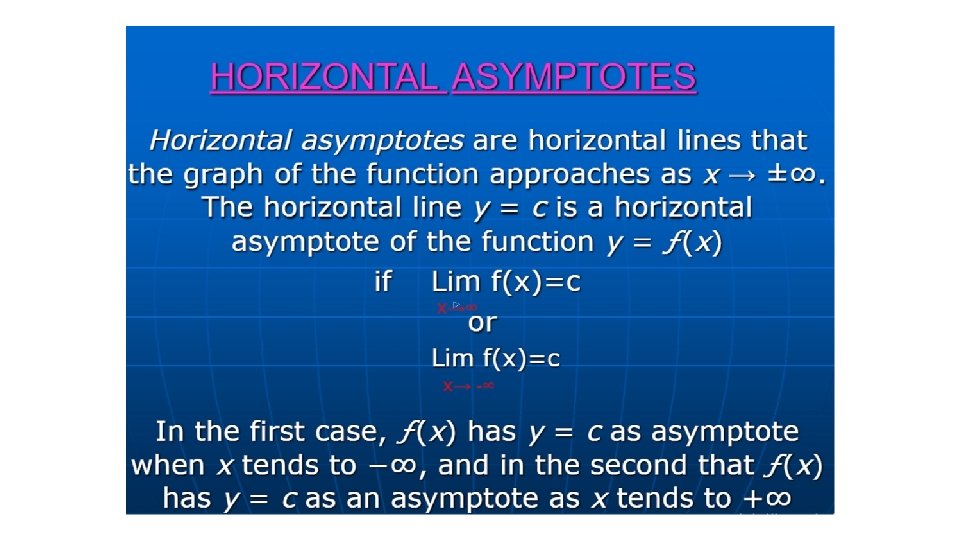
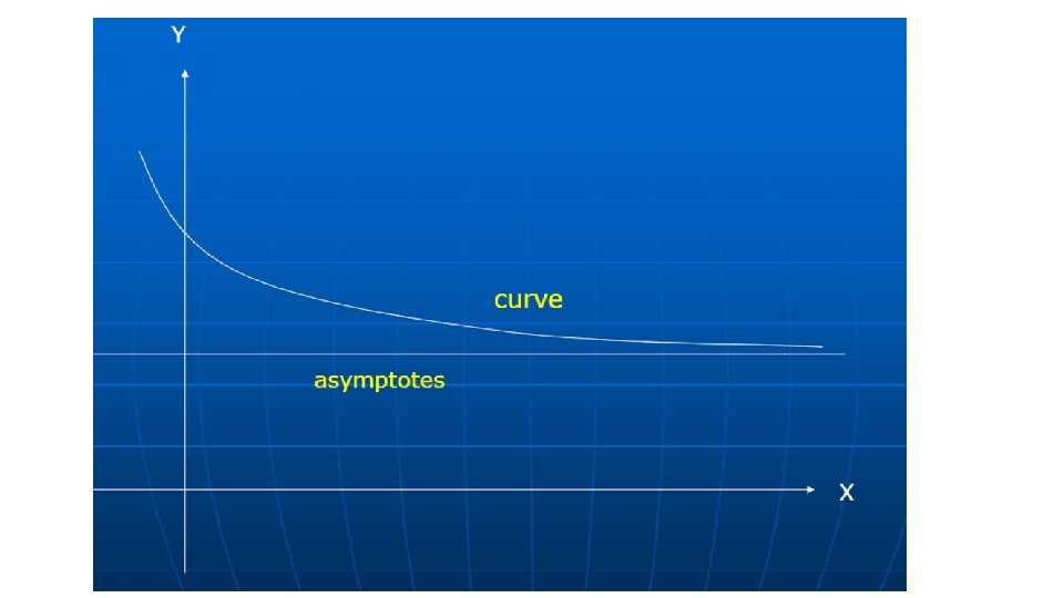
D. ASYMPTOTES—HORIZONTAL Recall that, if either or , then the line y = L is a horizontal asymptote of the curve y = f (x). § If it turns out that (or -∞), then we do not have an asymptote to the right. § Nevertheless, that is still useful information for sketching the curve.

D. ASYMPTOTES—VERTICAL For rational functions, you can locate the vertical asymptotes by equating the denominator to 0 after canceling any common factors. § However, for other functions, this method does not apply.

D. ASYMPTOTES—VERTICAL Furthermore, in sketching the curve, it is very useful to know exactly which of the statements is true. § If f(a) is not defined but a is an endpoint of the domain of f, then you should compute or , whether or not this limit is infinite.

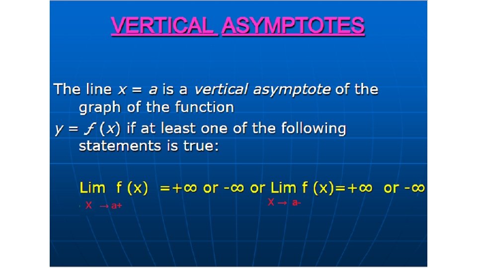
D. ASYMPTOTES—VERTICAL Recall that the line x = a is a vertical asymptote if at least one of the following statements is true:

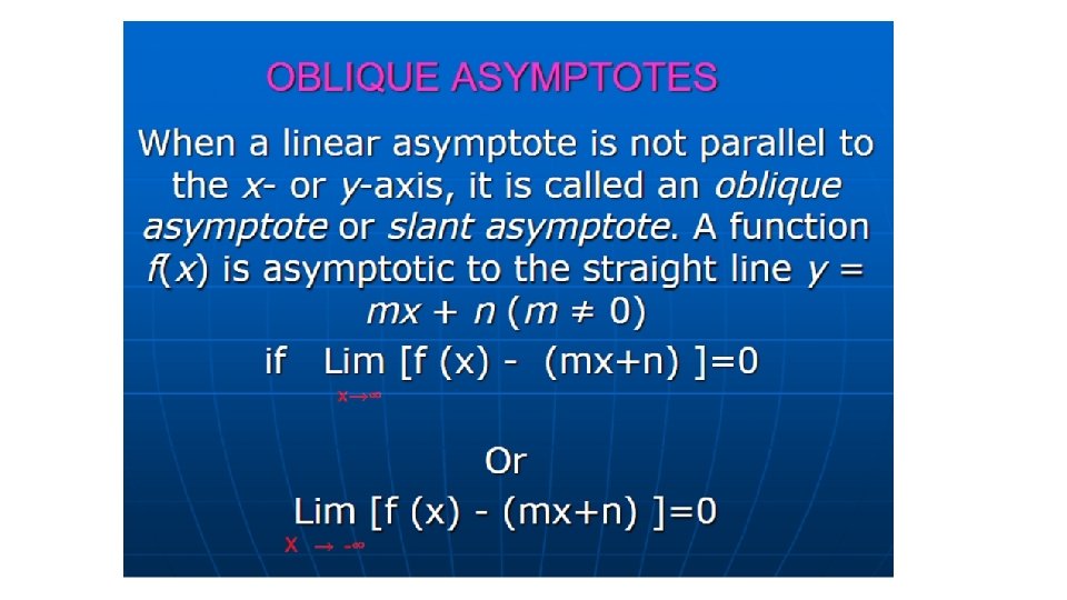
SLANT ASYMPTOTES Some curves have asymptotes that are oblique—that is, neither horizontal nor vertical.

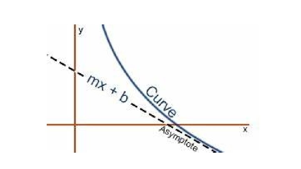
SLANT (OBLIQUE) ASYMPTOTES If , then the line y = mx + b is called a slant asymptote. § This is because the vertical distance between the curve y = f(x) and the line y = mx + b approaches 0. § A similar situation exists if we let x → -∞.

SLANT ASYMPTOTES For rational functions, slant asymptotes occur when the degree of the numerator is one more than the degree of the denominator. § In such a case, the equation of the slant asymptote can be found by long division— as in following example.

E. INTERVALS OF INCREASE OR DECREASE Use the I /D Test. Compute f’(x) and find the intervals on which: § f’(x) is positive (f is increasing). § f’(x) is negative (f is decreasing).

F. LOCAL MAXIMUM AND MINIMUM VALUES Find the critical numbers of f (the numbers c where f’(c) = 0 or f’(c) does not exist). Then, use the First Derivative Test. § If f’ changes from positive to negative at a critical number c, then f(c) is a local maximum. § If f’ changes from negative to positive at c, then f(c) is a local minimum.

F. LOCAL MAXIMUM AND MINIMUM VALUES Although it is usually preferable to use the First Derivative Test, you can use the Second Derivative Test if f’(c) = 0 and f’’(c) ≠ 0. Then, § f”(c) > 0 implies that f(c) is a local minimum. § f’’(c) < 0 implies that f(c) is a local maximum.

G. CONCAVITY AND POINTS OF INFLECTION Compute f’’(x) and use the Concavity Test. The curve is: § Concave upward where f’’(x) > 0 § Concave downward where f’’(x) < 0

G. CONCAVITY AND POINTS OF INFLECTION Inflection points occur where the direction of concavity changes.

H. SKETCH AND CURVE Using the information in items A–G, draw the graph. § Sketch the asymptotes as dashed lines. § Plot the intercepts, maximum and minimum points, and inflection points. § Then, make the curve pass through these points, rising and falling according to E, with concavity according to G, and approaching the asymptotes

H. SKETCH AND CURVE If additional accuracy is desired near any point, you can compute the value of the derivative there. § The tangent indicates the direction in which the curve proceeds.

A. DOMAIN • It’s often useful to start by determining the domain D of f. • This is the set of values of x for which f(x) is defined.

B. INTERCEPTS • The y-intercept is f(0) and this tells us where the curve intersects the y-axis. • To find the x-intercepts, we set y = 0 and solve for x. • You can omit this step if the equation is difficult to solve.

C. SYMMETRY—EVEN FUNCTION • If f(-x) = f(x) for all x in D, that is, the equation of the curve is unchanged when x is replaced by -x, then f is an even function and the curve is symmetric about the y-axis. • This means that our work is cut in half.

C. SYMMETRY—EVEN FUNCTION • If we know what the curve looks like for x ≥ 0, then we need only reflect about the y-axis to obtain the complete curve.

C. SYMMETRY—EVEN FUNCTION • Here are some examples: • • y = x 2 y = x 4 y = |x| y = cos x

C. SYMMETRY—ODD FUNCTION • If f(-x) = -f(x) for all x in D, then f is an odd function and the curve is symmetric about the origin.

C. SYMMETRY—ODD FUNCTION • Again, we can obtain the complete curve if we know what it looks like for x ≥ 0. • Rotate 180° about the origin.

C. SYMMETRY—ODD FUNCTION • Some simple examples of odd functions are: • • y=x y = x 3 y = x 5 y = sin x

C. SYMMETRY—PERIODIC FUNCTION • If f(x + p) = f(x) for all x in D, where p is a positive constant, then f is called a periodic function. • The smallest such number p is called the period. • For instance, y = sin x has period 2π and y = tan x has period π.

C. SYMMETRY—PERIODIC FUNCTION • If we know what the graph looks like in an interval of length p, then we can use translation to sketch the entire graph.

D. ASYMPTOTES—HORIZONTAL • Recall that, if either or , then the line y = L is a horizontal asymptote of the curve y = f (x). • If it turns out that (or -∞), then we do not have an asymptote to the right. • Nevertheless, that is still useful information for sketching the curve.

D. ASYMPTOTES—VERTICAL • Recall that the line x = a is a vertical asymptote if at least one of the following statements is true:

D. ASYMPTOTES—VERTICAL • For rational functions, you can locate the vertical asymptotes by equating the denominator to 0 after canceling any common factors. • However, for other functions, this method does not apply.

D. ASYMPTOTES—VERTICAL • Furthermore, in sketching the curve, it is very useful to know exactly which of the statements is true. • If f(a) is not defined but a is an endpoint of the domain of f, then you should compute or , whether or not this limit is infinite.

E. INTERVALS OF INCREASE OR DECREASE • Use the I /D Test. • Compute f’(x) and find the intervals on which: • f’(x) is positive (f is increasing). • f’(x) is negative (f is decreasing).

F. LOCAL MAXIMUM AND MINIMUM VALUES • Find the critical numbers of f (the numbers c where f’(c) = 0 or f’(c) does not exist). • Then, use the First Derivative Test. • If f’ changes from positive to negative at a critical number c, then f(c) is a local maximum. • If f’ changes from negative to positive at c, then f(c) is a local minimum.

F. LOCAL MAXIMUM AND MINIMUM VALUES • Although it is usually preferable to use the First Derivative Test, you can use the Second Derivative Test if f’(c) = 0 and f’’(c) ≠ 0. • Then, • f”(c) > 0 implies that f(c) is a local minimum. • f’’(c) < 0 implies that f(c) is a local maximum.

G. CONCAVITY AND POINTS OF INFLECTION • Compute f’’(x) and use the Concavity Test. • The curve is: • Concave upward where f’’(x) > 0 • Concave downward where f’’(x) < 0

G. CONCAVITY AND POINTS OF INFLECTION • Inflection points occur where the direction of concavity changes.

H. SKETCH AND CURVE • Using the information in items A–G, draw the graph. • Sketch the asymptotes as dashed lines. • Plot the intercepts, maximum and minimum points, and inflection points. • Then, make the curve pass through these points, rising and falling according to E, with concavity according to G, and approaching the asymptotes

H. SKETCH AND CURVE • If additional accuracy is desired near any point, you can compute the value of the derivative there. • The tangent indicates the direction in which the curve proceeds.

GUIDELINES • Use the guidelines to sketch the curve Example 1

GUIDELINES Example 1 • A. The domain is: {x | x 2 – 1 ≠ 0} = {x | x ≠ ± 1} = (-∞, -1) U (-1, -1) U (1, ∞) • B. The x- and y-intercepts are both 0.

GUIDELINES Example 1 • C. Since f(-x) = f(x), the function is even. • The curve is symmetric about the y-axis.

GUIDELINES Example 1 • D. Therefore, the line y = 2 is a horizontal asymptote.

GUIDELINES Example 1 • Since the denominator is 0 when x = ± 1, we compute the following limits: • Thus, the lines x = 1 and x = -1 are vertical asymptotes.

GUIDELINES • This information about limits and asymptotes enables us to draw the preliminary sketch, showing the parts of the curve near the asymptotes. Example 1

GUIDELINES Example 1 • E. • Since f’(x) > 0 when x < 0 (x ≠ 1) and f’(x) < 0 when x > 0 (x ≠ 1), f is: • Increasing on (-∞, -1) and (-1, 0) • Decreasing on (0, 1) and (1, ∞)

GUIDELINES Example 1 • F. The only critical number is x = 0. • Since f’ changes from positive to negative at 0, f(0) = 0 is a local maximum by the First Derivative Test.

GUIDELINES • G. • Since 12 x 2 + 4 > 0 for all x, we have • and Example 1

GUIDELINES Example 1 • Thus, the curve is concave upward on the intervals (-∞, -1) and (1, ∞) and concave downward on (-1, -1). • It has no point of inflection since 1 and -1 are not in the domain of f.

GUIDELINES • H. Using the information in E–G, we finish the sketch. Example 1

GUIDELINES • Sketch the graph of: Example 2

GUIDELINES • A. Domain = {x | x + 1 > 0} = {x | x > -1} = (-1, ∞) • B. The x- and y-intercepts are both 0. • C. Symmetry: None Example 2

GUIDELINES • D. Since Example 2 , there is no horizontal asymptote. • Since as x → -1+ and f(x) is always positive, we have , and so the line x = -1 is a vertical asymptote

GUIDELINES Example 2 • E. • We see that f’(x) = 0 when x = 0 (notice that -4/3 is not in the domain of f). • So, the only critical number is 0.

GUIDELINES Example 2 • As f’(x) < 0 when -1 < x < 0 and f’(x) > 0 when x > 0, f is: • Decreasing on (-1, 0) • Increasing on (0, ∞)

GUIDELINES Example 2 • F. Since f’(0) = 0 and f’ changes from negative to positive at 0, f(0) = 0 is a local (and absolute) minimum by the First Derivative Test.

GUIDELINES Example 2 • G. • Note that the denominator is always positive. • The numerator is the quadratic 3 x 2 + 8 x + 8, which is always positive because its discriminant is b 2 - 4 ac = -32, which is negative, and the coefficient of x 2 is positive.

GUIDELINES Example 2 • So, f”(x) > 0 for all x in the domain of f. • This means that: • f is concave upward on (-1, ∞). • There is no point of inflection.

GUIDELINES • H. The curve is sketched here. Example 2

GUIDELINES • Sketch the graph of: x f(x) = xe Example 3

GUIDELINES Example 3 • A. The domain is IR • B. The x- and y-intercepts are both 0. • C. Symmetry: None

GUIDELINES Example 3 • D. As both x and ex become large as x → ∞, we have • However, as x → -∞, ex → 0.

GUIDELINES Example 3 • So, we have an indeterminate product that requires the use of L’Hospital’s Rule: • Thus, the x-axis is a horizontal asymptote.

GUIDELINES Example 3 • E. f’(x) = xex + ex = (x + 1) ex • As ex is always positive, we see that f’(x) > 0 when x + 1 > 0, and f’(x) < 0 when x + 1 < 0. • So, f is: • Increasing on (-1, ∞) • Decreasing on (-∞, -1)

GUIDELINES Example 3 • F. Since f’(-1) = 0 and f’ changes from negative to positive at x = -1, f(-1) = -e-1 is a local (and absolute) minimum.

GUIDELINES Example 3 • G. f’’(x) = (x + 1)ex + ex = (x + 2)ex • f”(x) = 0 if x > -2 and f’’(x) < 0 if x < -2. • So, f is concave upward on (-2, ∞) and concave downward on ( -∞, -2). • The inflection point is (-2, -2 e-2)

GUIDELINES • H. We use this information to sketch the curve. Example 3

GUIDELINES • Sketch the graph of: Example 4

GUIDELINES Example 4 • A. The domain is IR • B. The y-intercept is f(0) = ½. The x-intercepts occur when cos x =0, that is, x = (2 n + 1)π/2, where n is an integer.

GUIDELINES Example 4 • C. f is neither even nor odd. • However, f(x + 2π) = f(x) for all x. • Thus, f is periodic and has period 2π. • So, in what follows, we need to consider only 0 ≤ x ≤ 2π and then extend the curve by translation in part H. • D. Asymptotes: None

GUIDELINES Example 4 • E. • Thus, f’(x) > 0 when 2 sin x + 1 < 0 7π/6 < x < 11π/6 sin x < -½

GUIDELINES • Thus, f is: • Increasing on (7π/6, 11π/6) • Decreasing on (0, 7π/6) and (11π/6, 2π) Example 4

GUIDELINES Example 4 • F. From part E and the First Derivative Test, we see that: • The local minimum value is f(7π/6) = -1/ • The local maximum value is f(11π/6) = +1/

GUIDELINES Example 4 • G. If we use the Quotient Rule again and simplify, we get: • (2 + sin x)3 > 0 and 1 – sin x ≥ 0 for all x. • So, we know that f’’(x) > 0 when cos x < 0, that is, π/2 < x < 3π/2.

GUIDELINES Example 4 • Thus, f is concave upward on (π/2, 3π/2) and concave downward on (0, π/2) and (3π/2, 2π). • The inflection points are (π/2, 0) and (3π/2, 0).

GUIDELINES • H. The graph of the function restricted to 0 ≤ x ≤ 2π is shown here. Example 4

GUIDELINES • Then, we extend it, using periodicity, to the complete graph here. Example 4

GUIDELINES Example 5 • Sketch the graph of: 2 y = ln(4 - x )

GUIDELINES Example 5 • A. The domain is: • {x | 4 − x 2 > 0} = {x | x 2 < 4} = {x | |x| < 2} = (− 2, 2)

Example 5 GUIDELINES • B. The y-intercept is: f(0) = ln 4 • To find the x-intercept, we set: y = ln(4 – x 2) = 0 • We know that ln 1 = 0. • So, we have 4 – x 2 = 1 x 2 = 3 • Therefore, the x-intercepts are:

GUIDELINES Example 5 • C. f(-x) = f(x) • Thus, • f is even. • The curve is symmetric about the y-axis.

GUIDELINES Example 5 • D. We look for vertical asymptotes at the endpoints of the domain. • Since 4 − x 2 → 0+ as x → 2 - and as x → 2+, we have: • Thus, the lines x = 2 and x = -2 are vertical asymptotes.

GUIDELINES Example 5 • E. • f’(x) > 0 when -2 < x < 0 and f’(x) < 0 when 0 < x < 2. • So, f is: • Increasing on (-2, 0) • Decreasing on (0, 2)

GUIDELINES Example 5 • F. The only critical number is x = 0. • As f’ changes from positive to negative at 0, f(0) = ln 4 is a local maximum by the First Derivative Test.

GUIDELINES Example 5 • G. • Since f”(x) < 0 for all x, the curve is concave downward on (-2, 2) and has no inflection point.

GUIDELINES • H. Using this information, we sketch the curve. Example 5

SLANT ASYMPTOTES • Some curves have asymptotes that are oblique—that is, neither horizontal nor vertical.

SLANT ASYMPTOTES • If , then the line y = mx + b is called a slant asymptote. • This is because the vertical distance between the curve y = f(x) and the line y = mx + b approaches 0. • A similar situation exists if we let x → -∞.

SLANT ASYMPTOTES • For rational functions, slant asymptotes occur when the degree of the numerator is one more than the degree of the denominator. • In such a case, the equation of the slant asymptote can be found by long division— as in following example.

SLANT ASYMPTOTES • Sketch the graph of: Example 6

SLANT ASYMPTOTES Example 6 • A. The domain is: R = (-∞, ∞) • B. The x- and y-intercepts are both 0. • C. As f(-x) = -f(x), f is odd and its graph is symmetric about the origin.

SLANT ASYMPTOTES Example 6 • Since x 2 + 1 is never 0, there is no vertical asymptote. • Since f(x) → ∞ as x → ∞ and f(x) → -∞ as x → - ∞, there is no horizontal asymptote.