Sketching complexity of graph cuts Alexandr Andoni joint

Sketching complexity of graph cuts Alexandr Andoni joint work with: Robi Krauthgamer, David Woodruff

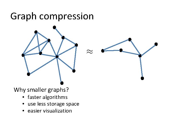
Graph compression Why smaller graphs? • faster algorithms • use less storage space • easier visualization

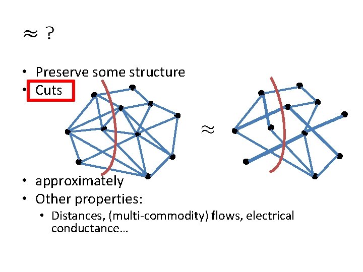
• Preserve some structure • Cuts • approximately • Other properties: • Distances, (multi-commodity) flows, electrical conductance…

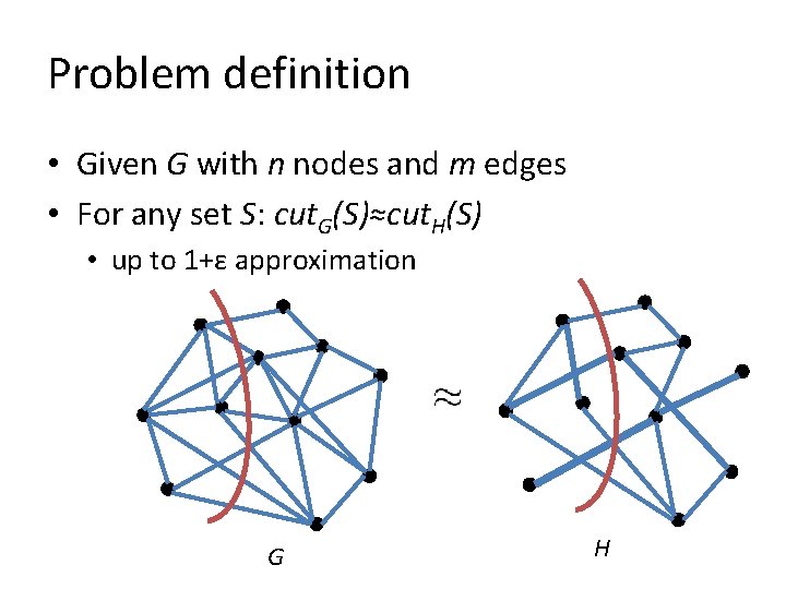
Problem definition • Given G with n nodes and m edges • For any set S: cut. G(S)≈cut. H(S) • up to 1+ε approximation G H

Cut sparsifiers • [Benczur-Karger’ 96]: • can construct graph H with O(n/ε 2 log n) edges • Approach: • sample edges in the graph • non-uniform sampling

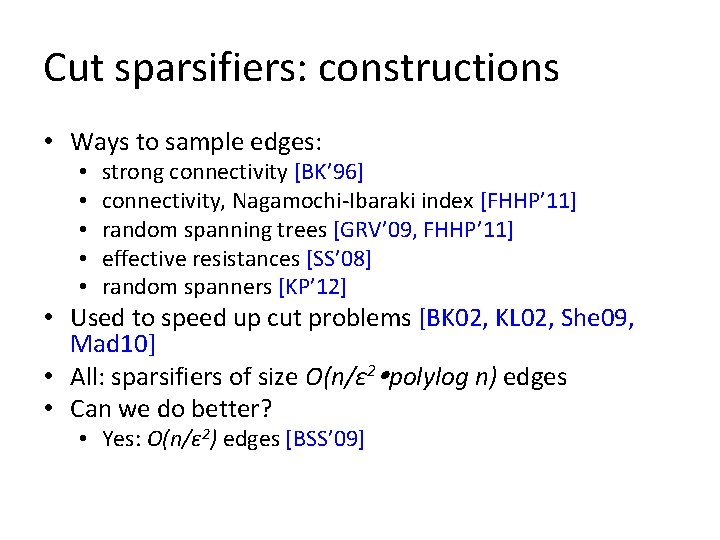
Cut sparsifiers: constructions • Ways to sample edges: • • • strong connectivity [BK’ 96] connectivity, Nagamochi-Ibaraki index [FHHP’ 11] random spanning trees [GRV’ 09, FHHP’ 11] effective resistances [SS’ 08] random spanners [KP’ 12] • Used to speed up cut problems [BK 02, KL 02, She 09, Mad 10] • All: sparsifiers of size O(n/ε 2 polylog n) edges • Can we do better? • Yes: O(n/ε 2) edges [BSS’ 09]

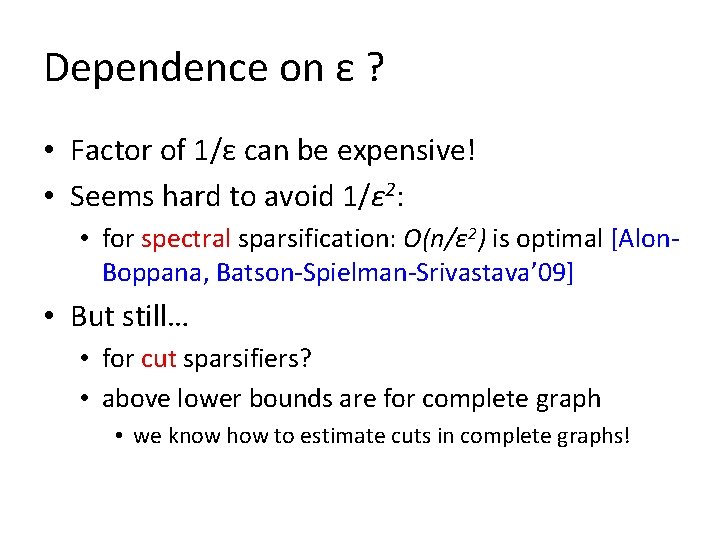
Dependence on ε ? • Factor of 1/ε can be expensive! • Seems hard to avoid 1/ε 2: • for spectral sparsification: O(n/ε 2) is optimal [Alon. Boppana, Batson-Spielman-Srivastava’ 09] • But still… • for cut sparsifiers? • above lower bounds are for complete graph • we know how to estimate cuts in complete graphs!

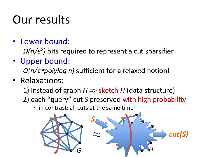
Our results • Lower bound: Ω(n/ε 2) bits required to represent a cut sparsifier • Upper bound: O(n/ε polylog n) sufficient for a relaxed notion! • Relaxations: 1) instead of graph H => sketch H (data structure) 2) each “query” cut S preserved with high probability • in contrast: all cuts at the same time S cut(S) G H

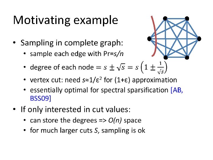
Motivating example •

Upper Bound • Three parts: i) sketch description ii) sketch size is O(n/ε log 2 n) iii) estimation algorithm, correctness • will focus on unweighted graphs

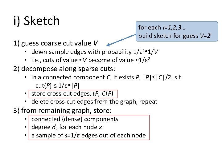
i) Sketch 1) guess coarse cut value V for each i=1, 2, 3… build sketch for guess V=2 i • down-sample edges with probability 1/ε 2 1/V • i. e. , cuts of value ≈V become of value ≈1/ε 2 2) decompose along sparse cuts: • in a connected component C, if exists P, |P|≤|C|/2, s. t. cut(P) ≤ 1/ε |P| • store cross-cut edges, (P, CP) • delete cross-cut edges from the graph, repeat 3) from remaining graph, store: • connected (dense) components • degree dx for each node x • a sample of s=1/ε edges out of each node

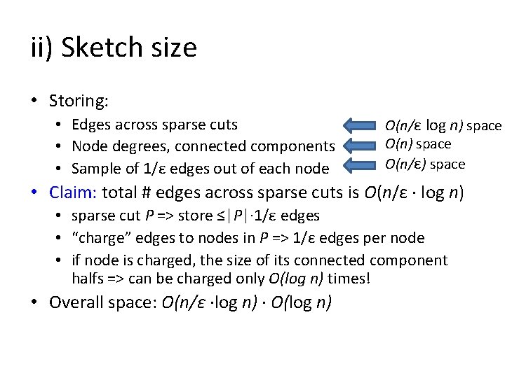
ii) Sketch size • Storing: • Edges across sparse cuts • Node degrees, connected components • Sample of 1/ε edges out of each node O(n/ε log n) space O(n/ε) space • Claim: total # edges across sparse cuts is O(n/ε · log n) • sparse cut P => store ≤|P|· 1/ε edges • “charge” edges to nodes in P => 1/ε edges per node • if node is charged, the size of its connected component halfs => can be charged only O(log n) times! • Overall space: O(n/ε ·log n) · O(log n)

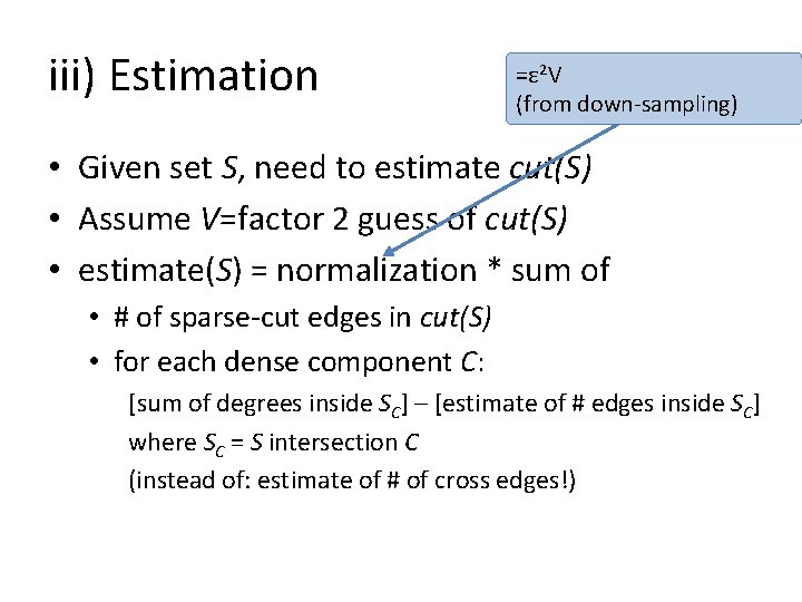
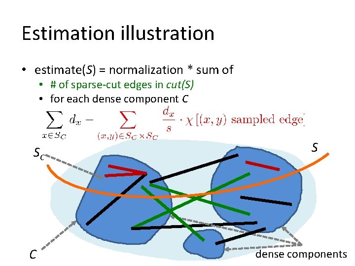
iii) Estimation =ε 2 V (from down-sampling) • Given set S, need to estimate cut(S) • Assume V=factor 2 guess of cut(S) • estimate(S) = normalization * sum of • # of sparse-cut edges in cut(S) • for each dense component C: [sum of degrees inside SC] – [estimate of # edges inside SC] where SC = S intersection C (instead of: estimate of # of cross edges!)

Estimation illustration • estimate(S) = normalization * sum of • # of sparse-cut edges in cut(S) • for each dense component C SC C S dense components

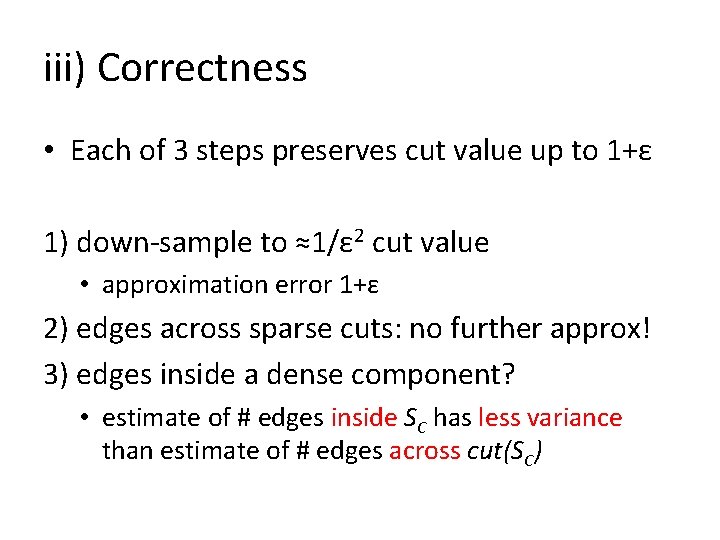
iii) Correctness • Each of 3 steps preserves cut value up to 1+ε 1) down-sample to ≈1/ε 2 cut value • approximation error 1+ε 2) edges across sparse cuts: no further approx! 3) edges inside a dense component? • estimate of # edges inside SC has less variance than estimate of # edges across cut(SC)

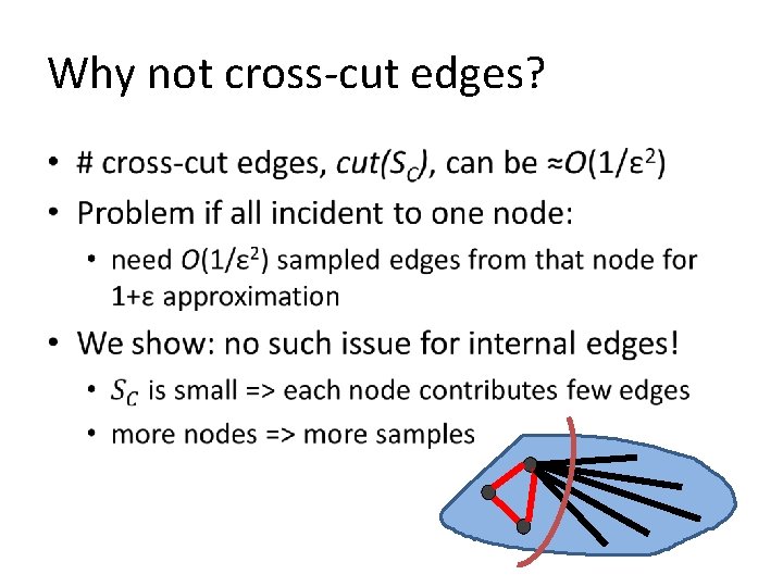
Why not cross-cut edges? •

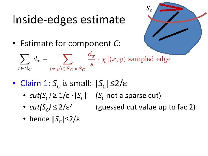
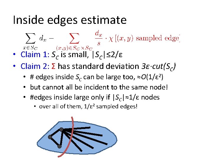
Inside-edges estimate SC • Estimate for component C: • Claim 1: SC is small: |SC|≤ 2/ε • cut(SC) ≥ 1/ε ·|SC| (SC not a sparse cut) • cut(SC) ≤ 2/ε 2 (guessed cut value up to fac 2) • hence |SC|≤ 2/ε

Inside edges estimate • Claim 1: SC is small, |SC|≤ 2/ε • Claim 2: Σ has standard deviation 3ε·cut(SC) • # edges inside SC can be large too, ≈O(1/ε 2) • but cannot all be incident to the same node! • #edges inside large only if |SC|≈1/ε nodes • over all of them, 1/ε 2 sampled edges!

Wrap-up of upper bound • Attentive variance calculation completes proof • 1+O(ε) multiplicative approximation by Chebyshev inequality • As usual: “high probability” by repeating logarithmic number of times • Construction time? • requires computing sparse cuts… NP-hard problem! • OK to compute approximate sparse cuts! • α-approximation => sketch size O(α · n/ε · log 2 n) • E. g. , using [Madry’ 10]: • O(mn 1+δ/ε) runtime for O(n/ε · polylog n) space

An application • Sketching for global min-cut • Theorem: can compute sketch(G), of size O(n/ε · polylog n) so that: • sketch(G 1), sketch(G 2) enough to compute global min-cut of G 1+G 2 • Obviously extends to >>2 partitions of graph • Previous approaches have 1/ε 2 dependence [AG 09, KL 13, AGM 12, GKK 10, GKP 12, KLMMS 14]

Sketching for global min-cut • Idea: • store two “cut sparsifiers”: 1) relaxed: O(n/ε · polylog n) space 2) classic, for 1. 5 -approximation: O(n· log n) space • Why enough? • [Karger’ 94]: only ≤n 3 cuts within 1. 5 of global min-cut • list ≤n 3 such cuts using (2) • for each, estimate up to 1+ε using (1) • In general: sketch good for polynomial # of (non-adaptive) queries

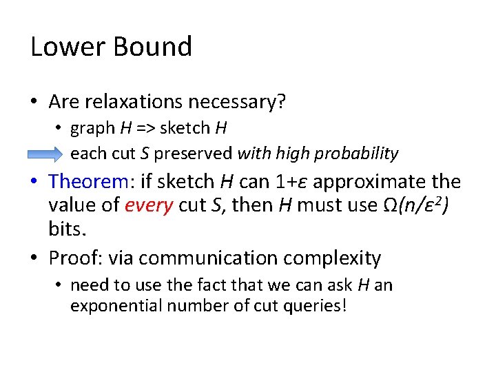
Lower Bound • Are relaxations necessary? • graph H => sketch H • each cut S preserved with high probability • Theorem: if sketch H can 1+ε approximate the value of every cut S, then H must use Ω(n/ε 2) bits. • Proof: via communication complexity • need to use the fact that we can ask H an exponential number of cut queries!

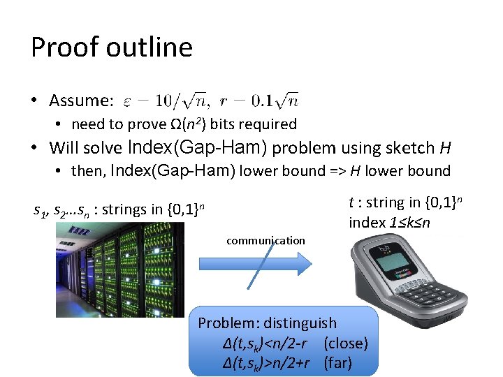
Proof outline • Assume: • need to prove Ω(n 2) bits required • Will solve Index(Gap-Ham) problem using sketch H • then, Index(Gap-Ham) lower bound => H lower bound s 1, s 2…sn t : string in {0, 1}n index 1≤k≤n : strings in {0, 1}n communication Problem: distinguish Δ(t, sk)<n/2 -r (close) Δ(t, sk)>n/2+r (far)

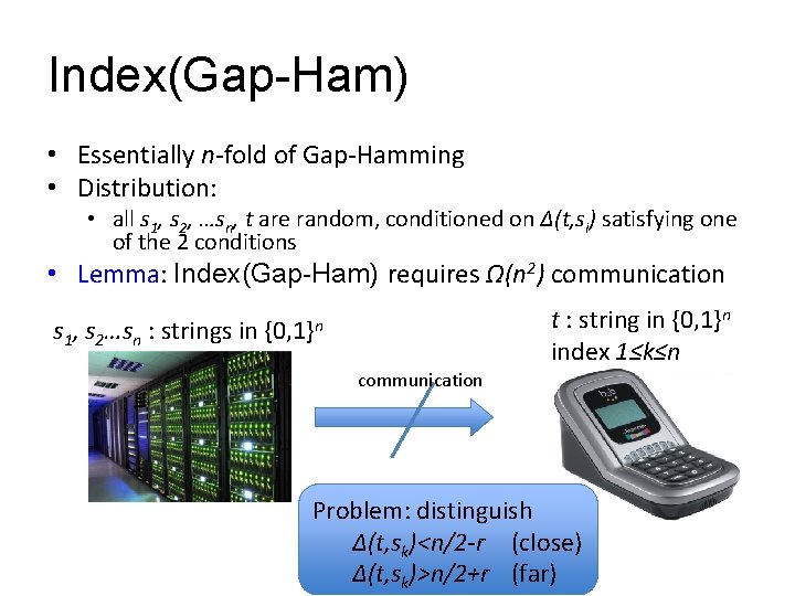
Index(Gap-Ham) • Essentially n-fold of Gap-Hamming • Distribution: • all s 1, s 2, …sn, t are random, conditioned on Δ(t, si) satisfying one of the 2 conditions • Lemma: Index(Gap-Ham) requires Ω(n 2) communication s 1, s 2…sn t : string in {0, 1}n index 1≤k≤n : strings in {0, 1}n communication Problem: distinguish Δ(t, sk)<n/2 -r (close) Δ(t, sk)>n/2+r (far)

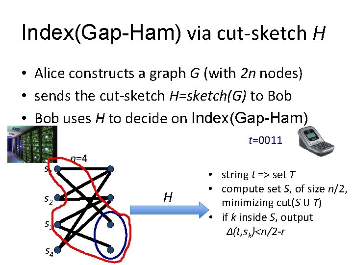
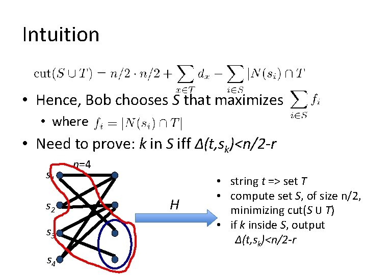
Index(Gap-Ham) via cut-sketch H • Alice constructs a graph G (with 2 n nodes) • sends the cut-sketch H=sketch(G) to Bob • Bob uses H to decide on Index(Gap-Ham) t=0011 s 2 s 3 s 4 n=4 H • string t => set T • compute set S, of size n/2, minimizing cut(S U T) • if k inside S, output Δ(t, sk)<n/2 -r

Intuition • Hence, Bob chooses S that maximizes • where • Need to prove: k in S iff Δ(t, sk)<n/2 -r s 1 s 2 s 3 s 4 n=4 H • string t => set T • compute set S, of size n/2, minimizing cut(S U T) • if k inside S, output Δ(t, sk)<n/2 -r

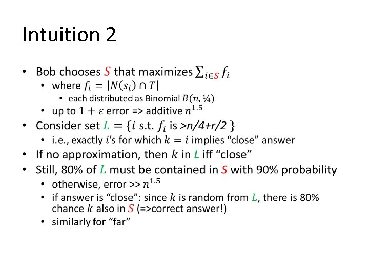
Intuition 2 •

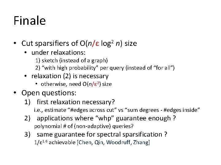
Finale • Cut sparsifiers of O(n/ε log 2 n) size • under relaxations: 1) sketch (instead of a graph) 2) “with high probability” per query (instead of “for all”) • relaxation (2) is necessary • otherwise, need O(n/ε 2) size • Open questions: 1) first relaxation necessary? i. e. , estimate “#edges across cut” vs “sum degrees - #edges inside” 2) applications where “whp” guarantee enough ? polynomial # of (non-adaptive) queries? 3) same guarantee for spectral sparsification ? 1/ε 1. 6 achievable [Chen, Qin, Woodruff, Zhang]