Sketching as a Tool for Numerical Linear Algebra

Sketching as a Tool for Numerical Linear Algebra All Lectures David Woodruff IBM Almaden

Massive data sets Examples § Internet traffic logs § Financial data § etc. Algorithms § Want nearly linear time or less § Usually at the cost of a randomized approximation 2

Regression analysis Regression § Statistical method to study dependencies between variables in the presence of noise. 3

Regression analysis Linear Regression § Statistical method to study linear dependencies between variables in the presence of noise. 4

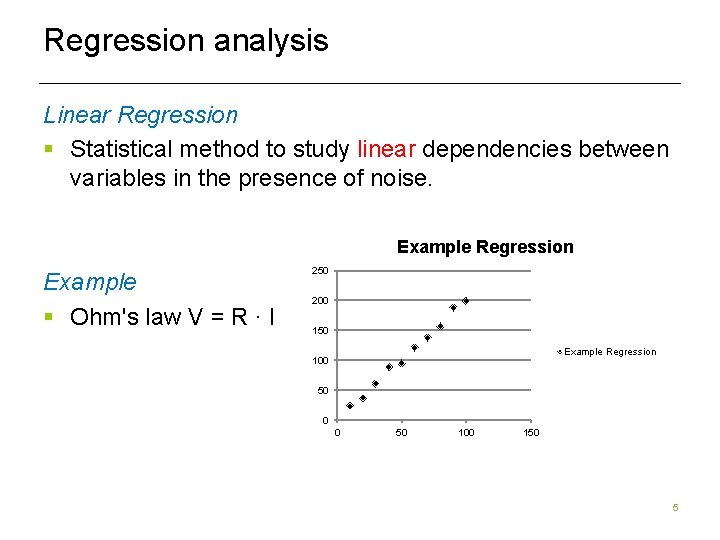
Regression analysis Linear Regression § Statistical method to study linear dependencies between variables in the presence of noise. Example Regression Example § Ohm's law V = R ∙ I 250 200 150 Example Regression 100 50 0 0 50 100 150 5

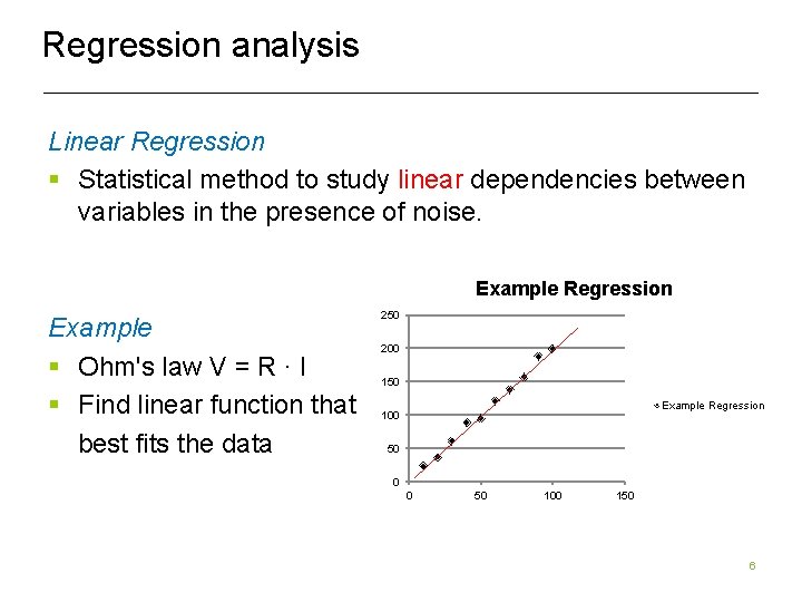
Regression analysis Linear Regression § Statistical method to study linear dependencies between variables in the presence of noise. Example Regression Example § Ohm's law V = R ∙ I § Find linear function that best fits the data 250 200 150 Example Regression 100 50 0 0 50 100 150 6

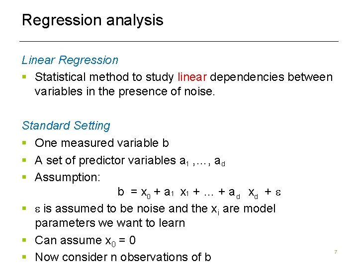
Regression analysis Linear Regression § Statistical method to study linear dependencies between variables in the presence of noise. Standard Setting § One measured variable b § A set of predictor variables a , …, a 1 d § Assumption: b = x + a x + … + a x + e 1 1 0 d d § e is assumed to be noise and the xi are model parameters we want to learn § Can assume x 0 = 0 § Now consider n observations of b 7

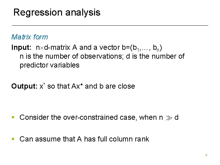
Regression analysis Matrix form Input: n d-matrix A and a vector b=(b 1, …, bn) n is the number of observations; d is the number of predictor variables Output: x* so that Ax* and b are close § Consider the over-constrained case, when n À d § Can assume that A has full column rank 8

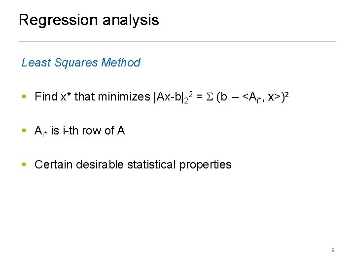
Regression analysis Least Squares Method § Find x* that minimizes |Ax-b|22 = S (bi – <Ai*, x>)² § Ai* is i-th row of A § Certain desirable statistical properties 9

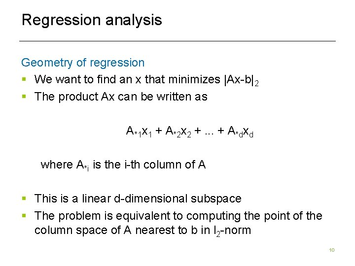
Regression analysis Geometry of regression § We want to find an x that minimizes |Ax-b|2 § The product Ax can be written as A*1 x 1 + A*2 x 2 +. . . + A*dxd where A*i is the i-th column of A § This is a linear d-dimensional subspace § The problem is equivalent to computing the point of the column space of A nearest to b in l 2 -norm 10

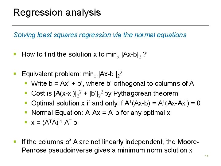
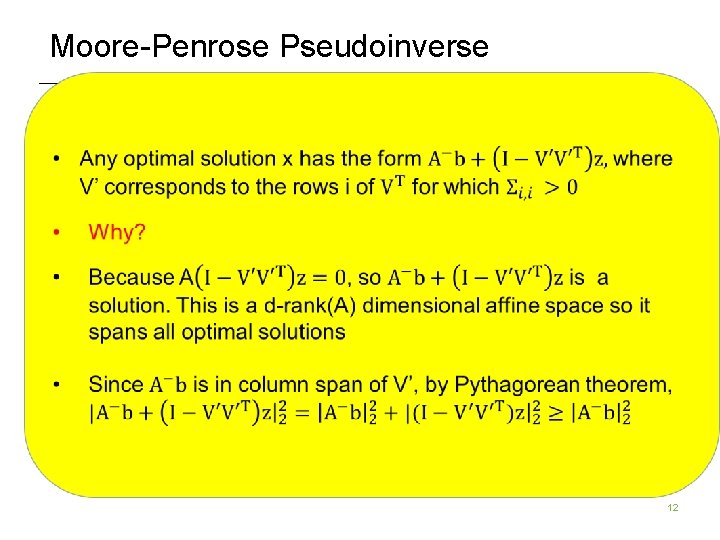
Regression analysis Solving least squares regression via the normal equations § How to find the solution x to minx |Ax-b|2 ? § Equivalent problem: minx |Ax-b |22 § Write b = Ax’ + b’, where b’ orthogonal to columns of A § Cost is |A(x-x’)|22 + |b’|22 by Pythagorean theorem § Optimal solution x if and only if AT(Ax-b) = AT(Ax-Ax’) = 0 § Normal Equation: ATAx = ATb for any optimal x § x = (ATA)-1 AT b § If the columns of A are not linearly independent, the Moore. Penrose pseudoinverse gives a minimum norm solution x 11

Moore-Penrose Pseudoinverse 12

Time Complexity 13

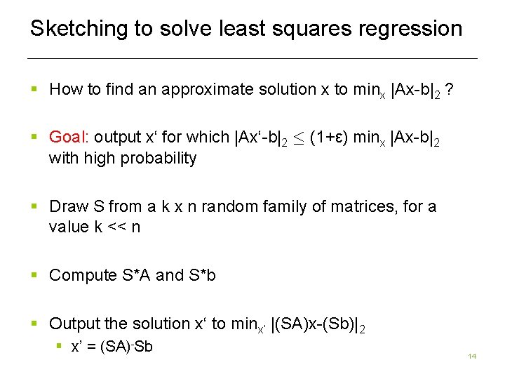
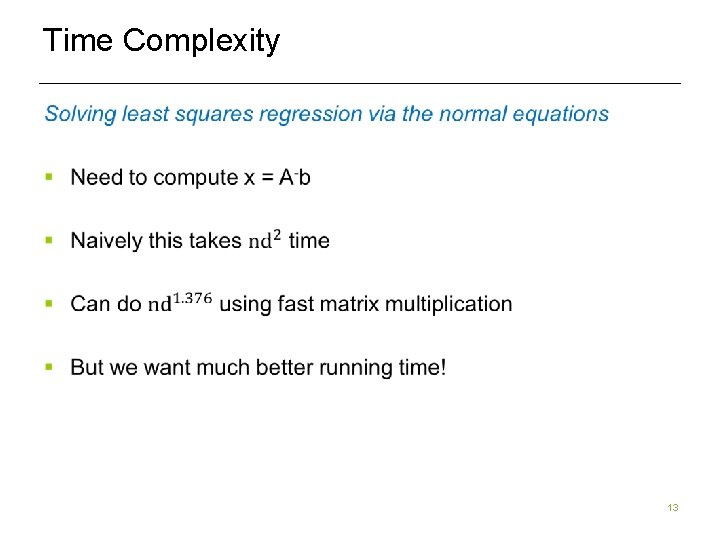
Sketching to solve least squares regression § How to find an approximate solution x to minx |Ax-b|2 ? § Goal: output x‘ for which |Ax‘-b|2 · (1+ε) minx |Ax-b|2 with high probability § Draw S from a k x n random family of matrices, for a value k << n § Compute S*A and S*b § Output the solution x‘ to minx‘ |(SA)x-(Sb)|2 § x’ = (SA)-Sb 14

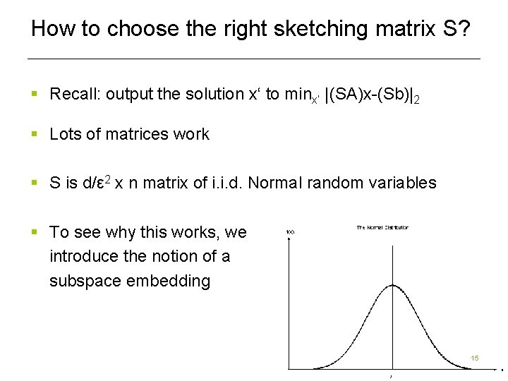
How to choose the right sketching matrix S? § Recall: output the solution x‘ to minx‘ |(SA)x-(Sb)|2 § Lots of matrices work § S is d/ε 2 x n matrix of i. i. d. Normal random variables § To see why this works, we introduce the notion of a subspace embedding 15

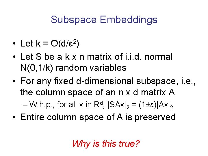
Subspace Embeddings • Let k = O(d/ε 2) • Let S be a k x n matrix of i. i. d. normal N(0, 1/k) random variables • For any fixed d-dimensional subspace, i. e. , the column space of an n x d matrix A – W. h. p. , for all x in Rd, |SAx|2 = (1±ε)|Ax|2 • Entire column space of A is preserved Why is this true?

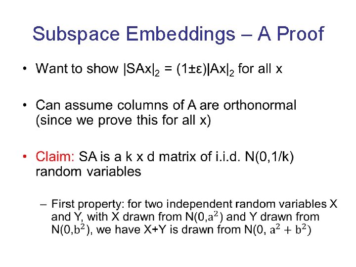
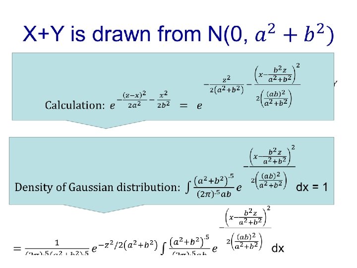
Subspace Embeddings – A Proof •

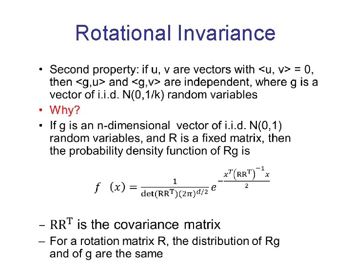
Rotational Invariance •

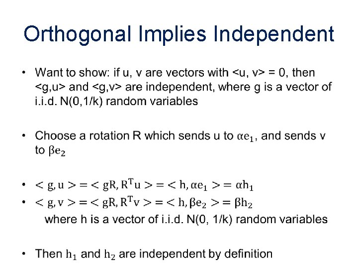
Orthogonal Implies Independent •

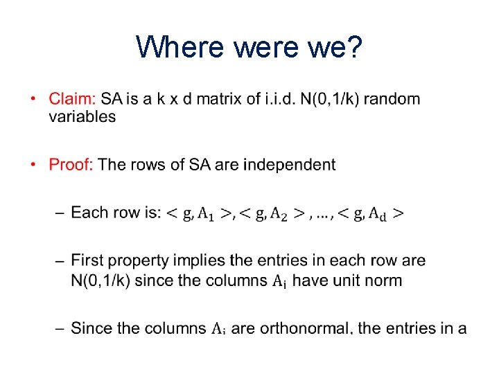
Where we? •

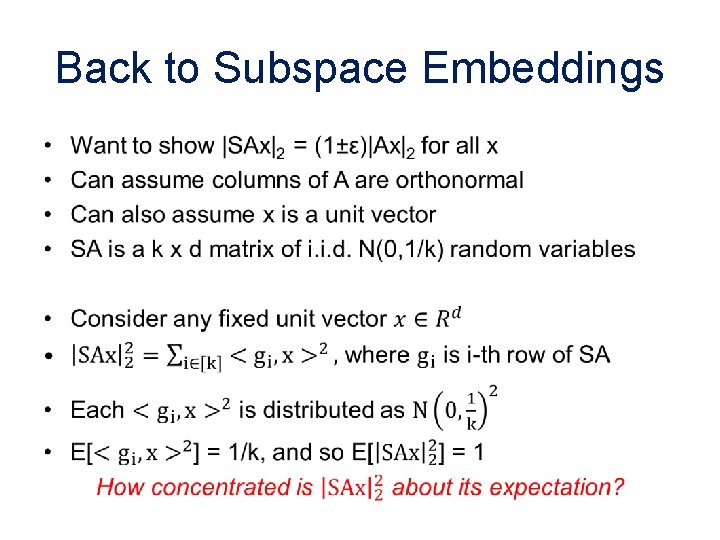
Back to Subspace Embeddings •

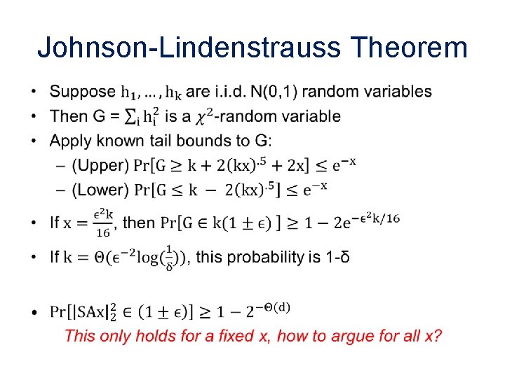
Johnson-Lindenstrauss Theorem •

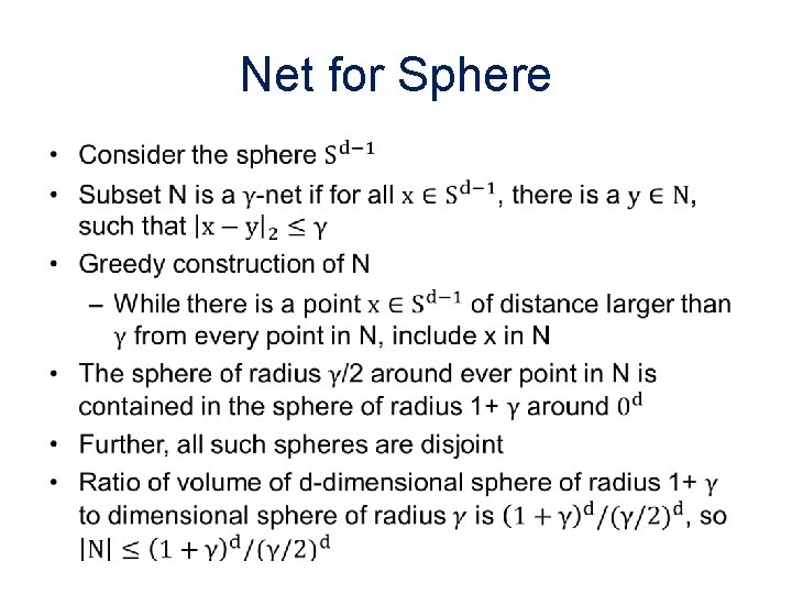
Net for Sphere •

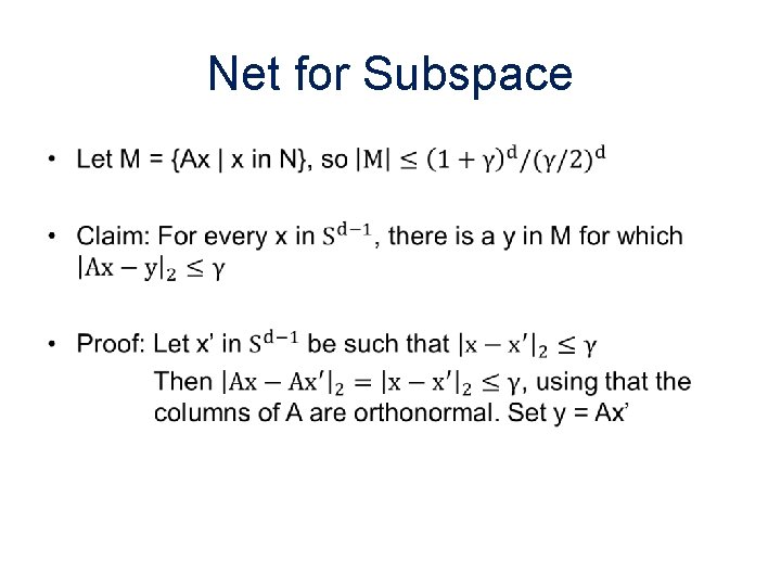
Net for Subspace •

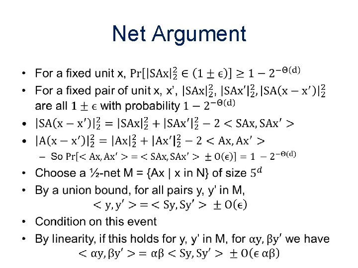
Net Argument •

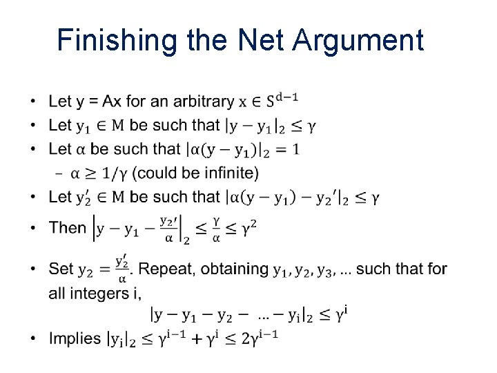
Finishing the Net Argument •

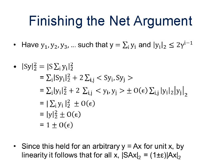
Finishing the Net Argument •

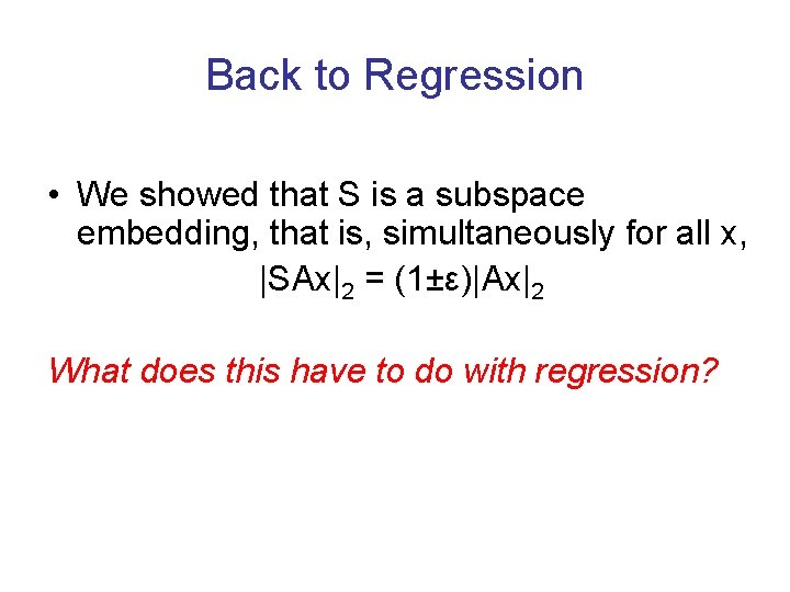
Back to Regression • We showed that S is a subspace embedding, that is, simultaneously for all x, |SAx|2 = (1±ε)|Ax|2 What does this have to do with regression?

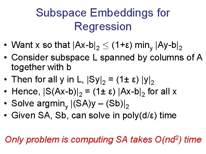
Subspace Embeddings for Regression • Want x so that |Ax-b|2 · (1+ε) miny |Ay-b|2 • Consider subspace L spanned by columns of A together with b • Then for all y in L, |Sy|2 = (1± ε) |y|2 • Hence, |S(Ax-b)|2 = (1± ε) |Ax-b|2 for all x • Solve argminy |(SA)y – (Sb)|2 • Given SA, Sb, can solve in poly(d/ε) time Only problem is computing SA takes O(nd 2) time

How to choose the right sketching matrix S? [S] § S is a Subsampled Randomized Hadamard Transform § S = P*H*D § D is a diagonal matrix with +1, -1 on diagonals § H is the Hadamard transform § P just chooses a random (small) subset of rows of H*D § S*A can be computed in O(nd log n) time Why does it work? 31

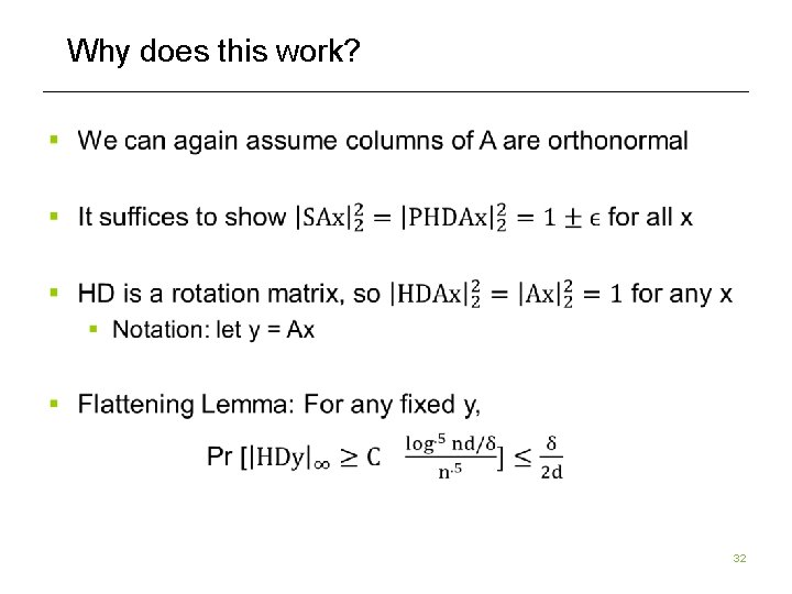
Why does this work? 32

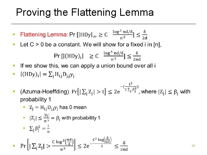
Proving the Flattening Lemma 33

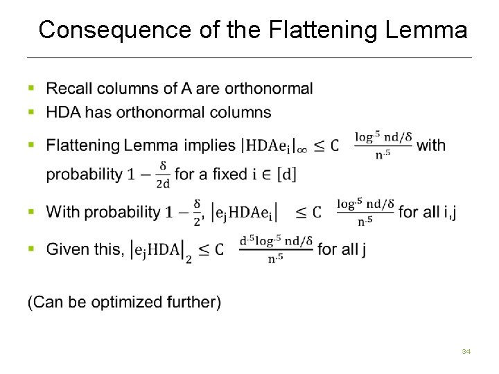
Consequence of the Flattening Lemma 34

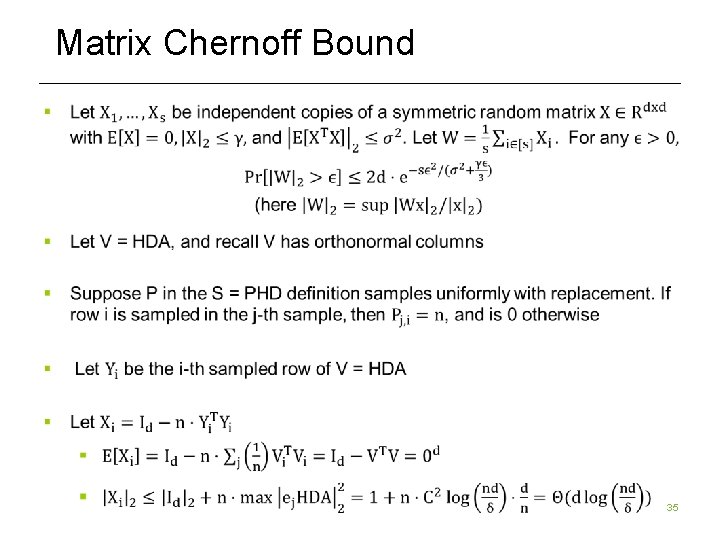
Matrix Chernoff Bound 35

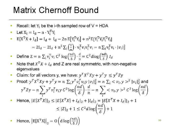
Matrix Chernoff Bound 36

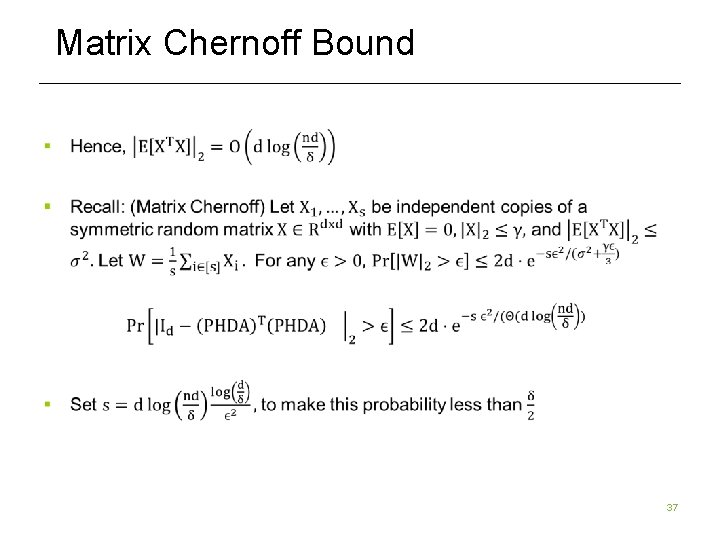
Matrix Chernoff Bound 37

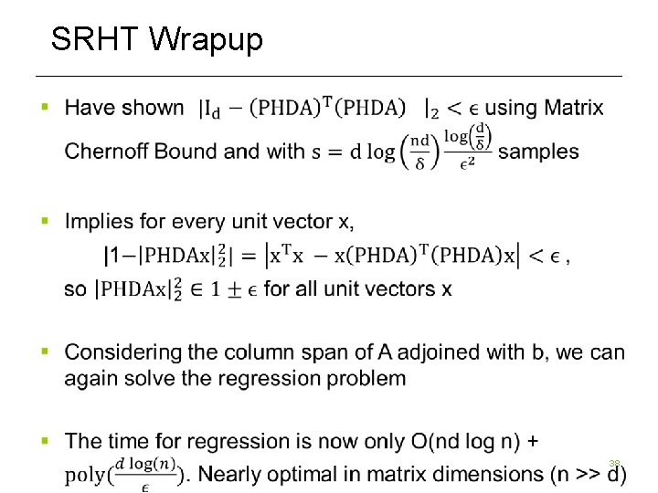
SRHT Wrapup 38

Faster Subspace Embeddings S [CW, MM, NN] § Count. Sketch matrix § Define k x n matrix S, for k = O(d 2/ε 2) § S is really sparse: single randomly chosen non-zero entry per column [ [ 0 0 1 0 0 0 0 0 -1 1 0 -1 0 0 0 0 0 1 § nnz(A) is number of non-zero entries of A 39

Simple Proof [Nguyen] § 40

Matrix Product Result [Kane, Nelson] § 41

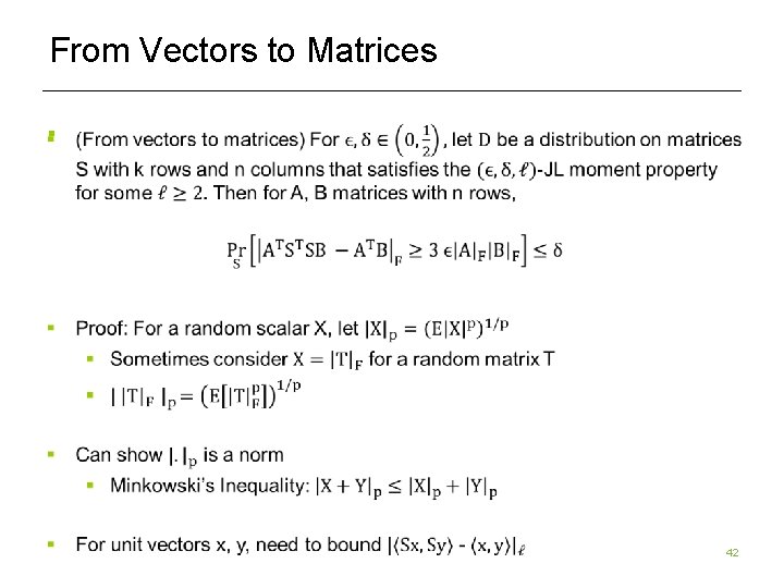
From Vectors to Matrices § 42

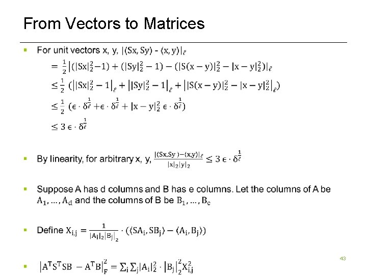
From Vectors to Matrices § 43

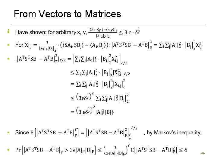
From Vectors to Matrices § 44

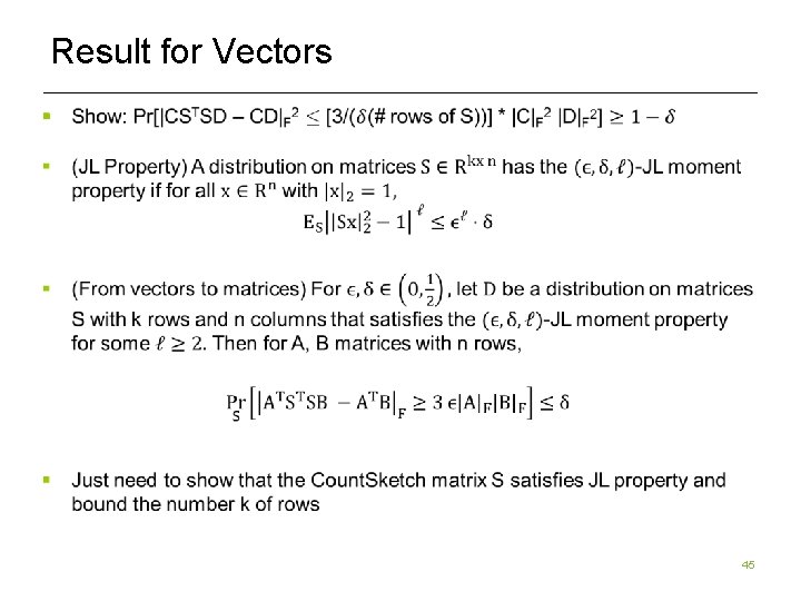
Result for Vectors § 45

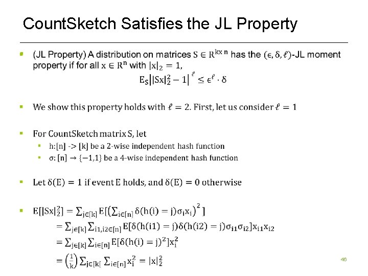
Count. Sketch Satisfies the JL Property § 46

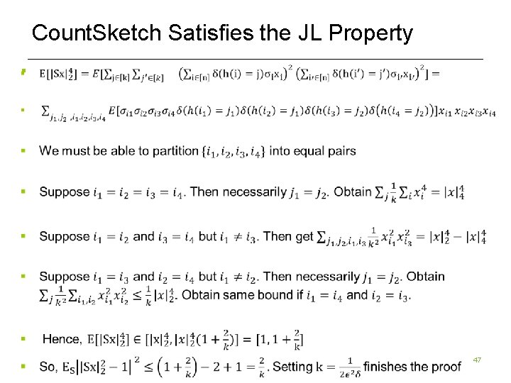
Count. Sketch Satisfies the JL Property § 47

Where are we? § 48

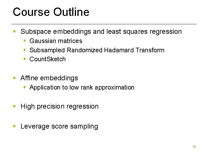
Course Outline § Subspace embeddings and least squares regression § Gaussian matrices § Subsampled Randomized Hadamard Transform § Count. Sketch § Affine embeddings § Application to low rank approximation § High precision regression § Leverage score sampling 49

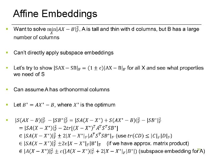
Affine Embeddings § 50

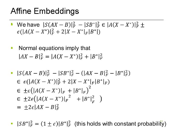
Affine Embeddings § 51

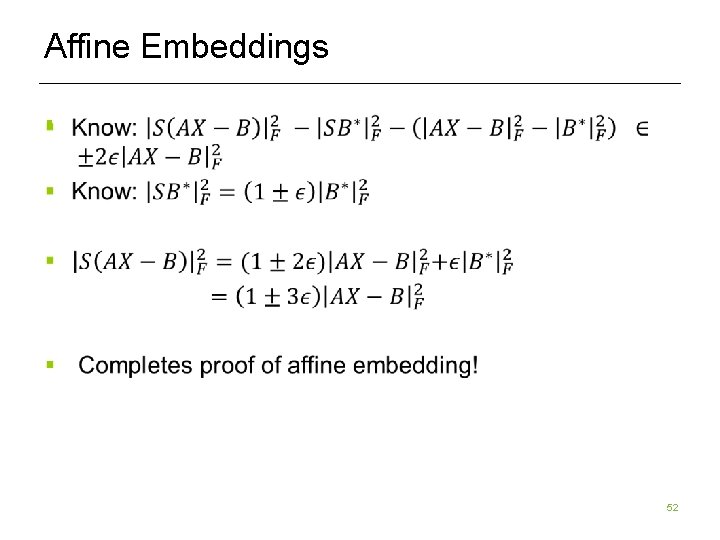
Affine Embeddings § 52

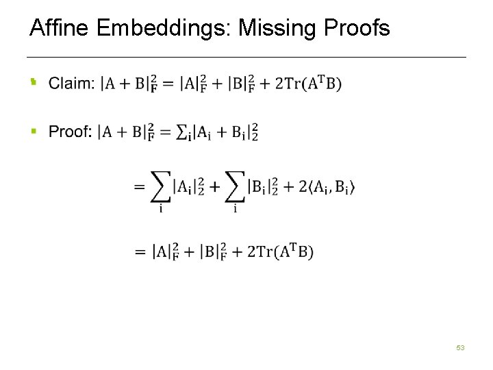
Affine Embeddings: Missing Proofs § 53

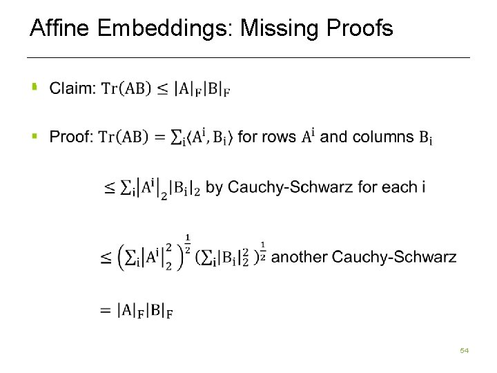
Affine Embeddings: Missing Proofs § 54

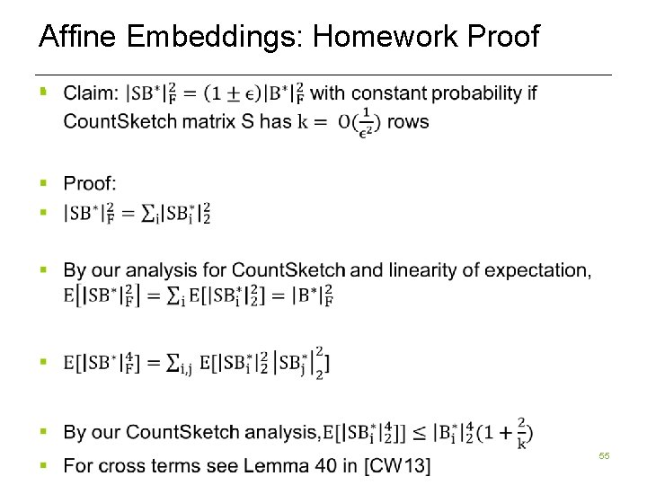
Affine Embeddings: Homework Proof § 55

Low rank approximation § A is an n x d matrix § Think of n points in Rd § E. g. , A is a customer-product matrix § Ai, j = how many times customer i purchased item j § A is typically well-approximated by low rank matrix § E. g. , high rank because of noise § Goal: find a low rank matrix approximating A § Easy to store, data more interpretable 56

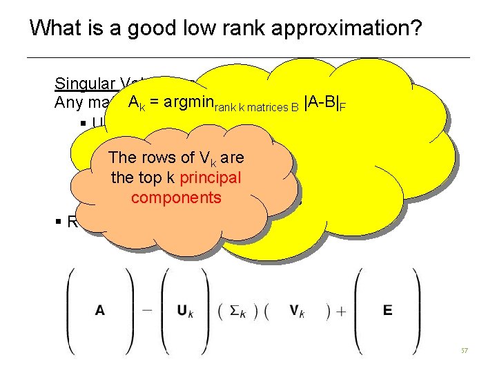
What is a good low rank approximation? Singular Value Decomposition (SVD) Ak = argminrank k matrices B |A-B|F Any matrix A = U ¢ Σ ¢ V § U has orthonormal columns § Σ is diagonal with non-increasing positive 2 1/2 ) (|C|F = (Σi, j C are i, j ) The rows of V k entries down the diagonal the top k principal § V has orthonormal rows components k exactly is Computing A expensive § Rank-k approximation: A k = Uk ¢ Σk ¢ Vk 57

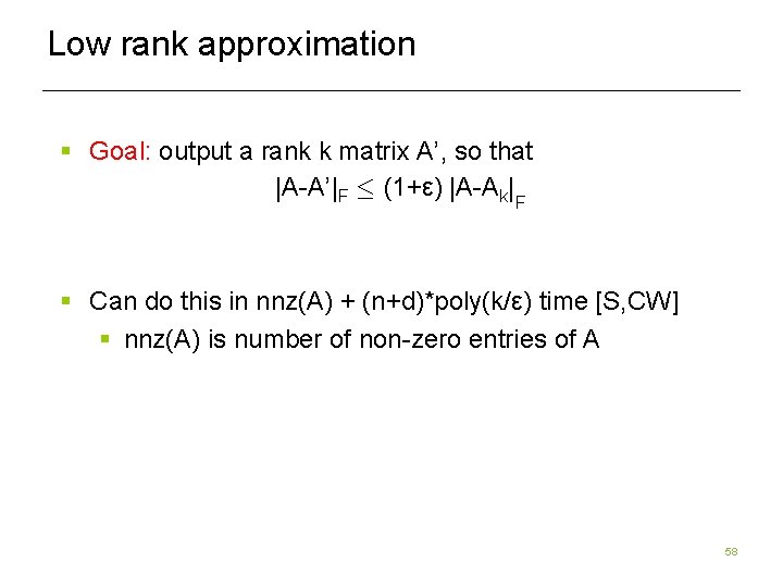
Low rank approximation § Goal: output a rank k matrix A’, so that |A-A’|F · (1+ε) |A-Ak|F § Can do this in nnz(A) + (n+d)*poly(k/ε) time [S, CW] § nnz(A) is number of non-zero entries of A 58

Solution to low-rank approximation [S] § Given n x d input matrix A § Compute S*A using a random matrix S with k/ε << n rows. S*A takes random linear combinations of rows of A A SA § Project rows of A onto SA, then find best rank-k approximation to points inside of SA. 59

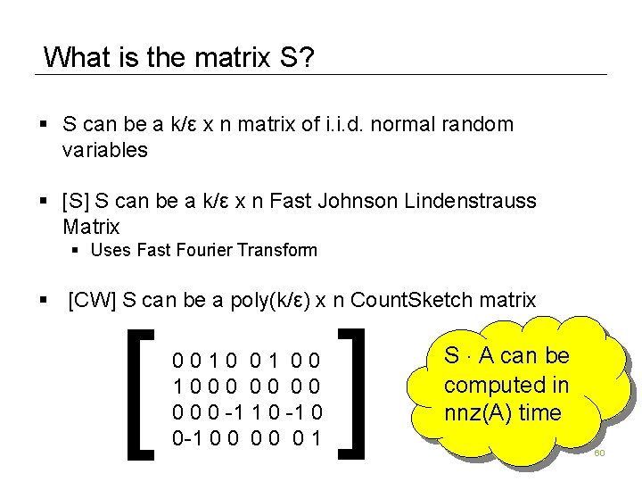
What is the matrix S? § S can be a k/ε x n matrix of i. i. d. normal random variables § [S] S can be a k/ε x n Fast Johnson Lindenstrauss Matrix § Uses Fast Fourier Transform § [CW] S can be a poly(k/ε) x n Count. Sketch matrix [ [ 0 0 1 0 0 0 0 0 -1 1 0 -1 0 0 0 0 0 1 S ¢ A can be computed in nnz(A) time 60

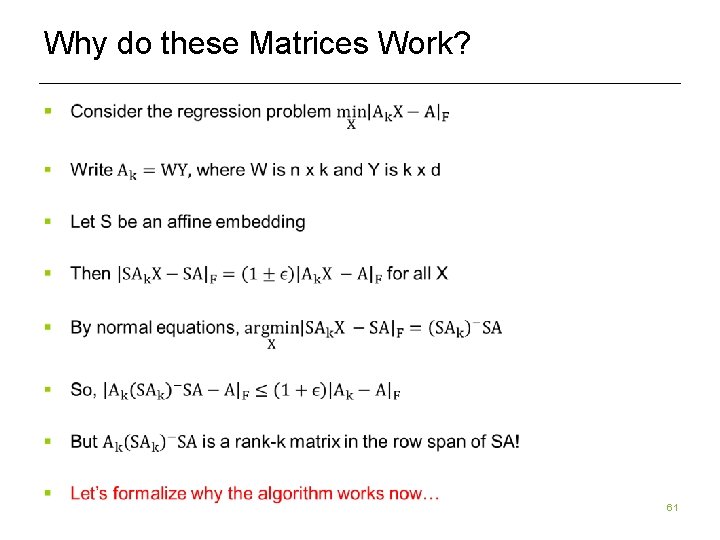
Why do these Matrices Work? § 61

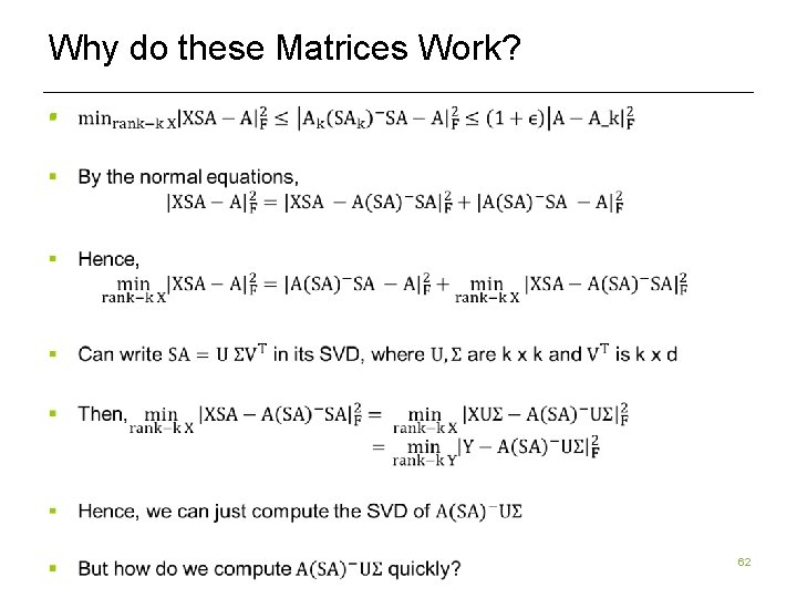
Why do these Matrices Work? § 62

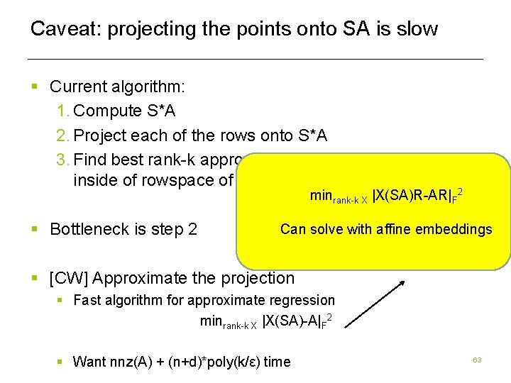
Caveat: projecting the points onto SA is slow § Current algorithm: 1. Compute S*A 2. Project each of the rows onto S*A 3. Find best rank-k approximation of projected points inside of rowspace of S*A minrank-k X |X(SA)R-AR|F 2 § Bottleneck is step 2 Can solve with affine embeddings § [CW] Approximate the projection § Fast algorithm for approximate regression minrank-k X |X(SA)-A|F 2 § Want nnz(A) + (n+d)*poly(k/ε) time 63

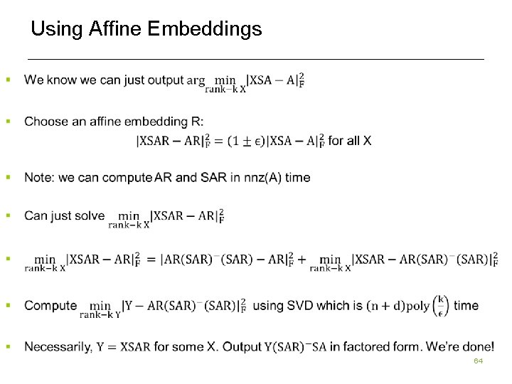
Using Affine Embeddings 64

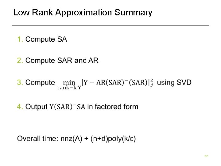
Low Rank Approximation Summary 65

Course Outline § Subspace embeddings and least squares regression § Gaussian matrices § Subsampled Randomized Hadamard Transform § Count. Sketch § Affine embeddings § Application to low rank approximation § High precision regression § Leverage score sampling 66

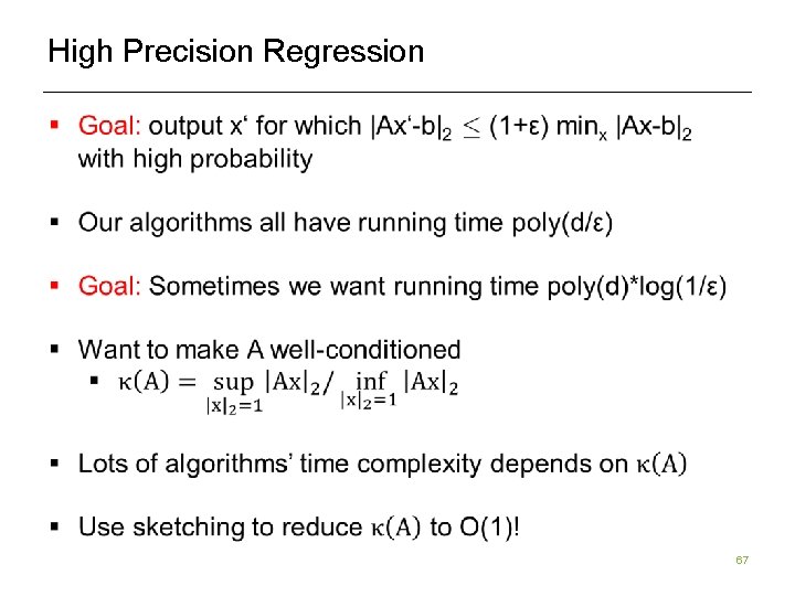
High Precision Regression 67

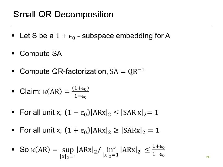
Small QR Decomposition 68

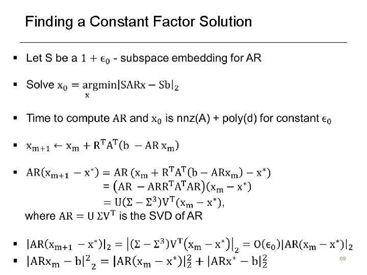
Finding a Constant Factor Solution 69

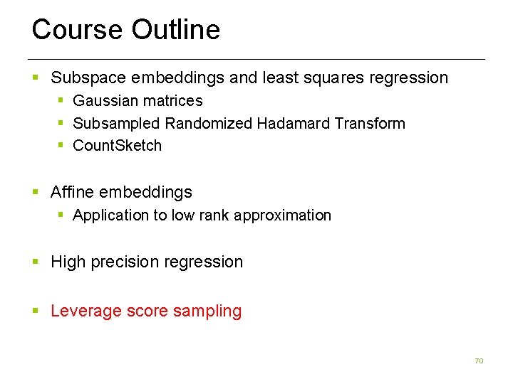
Course Outline § Subspace embeddings and least squares regression § Gaussian matrices § Subsampled Randomized Hadamard Transform § Count. Sketch § Affine embeddings § Application to low rank approximation § High precision regression § Leverage score sampling 70

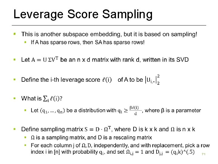
Leverage Score Sampling § 71

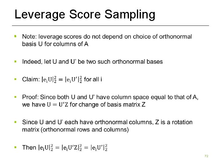
Leverage Score Sampling § 72

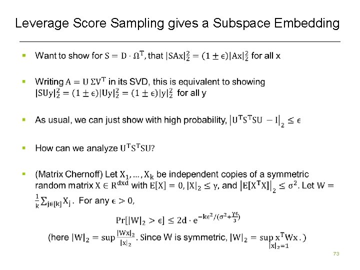
Leverage Score Sampling gives a Subspace Embedding § 73

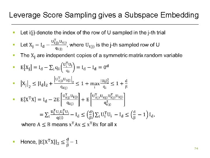
Leverage Score Sampling gives a Subspace Embedding § 74

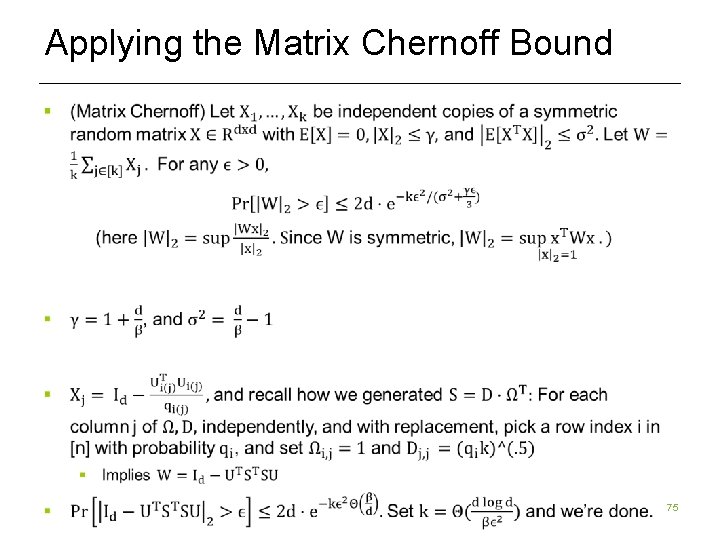
Applying the Matrix Chernoff Bound § 75

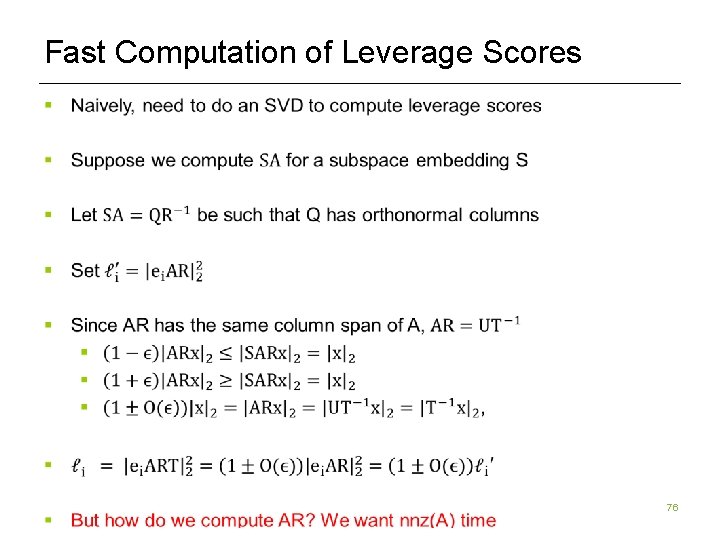
Fast Computation of Leverage Scores § 76

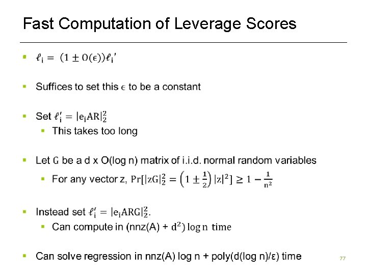
Fast Computation of Leverage Scores § 77

Course Outline § Subspace embeddings and least squares regression § Gaussian matrices § Subsampled Randomized Hadamard Transform § Count. Sketch § Affine embeddings § Application to low rank approximation § High precision regression § Leverage score sampling § Distributed Low Rank Approximation 78

Distributed low rank approximation § We have fast algorithms for low rank approximation, but can they be made to work in a distributed setting? § Matrix A distributed among s servers § For t = 1, …, s, we get a customer-product matrix from the t-th shop stored in server t. Server t’s matrix = At § Customer-product matrix A = A 1 + A 2 + … + As § Model is called the arbitrary partition model § More general than the row-partition model in which each customer shops in only one shop 79

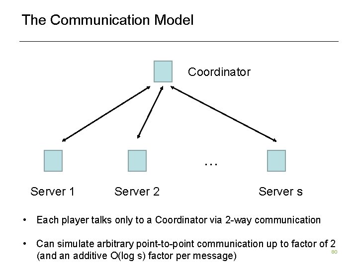
The Communication Model Coordinator … Server 1 Server 2 Server s • Each player talks only to a Coordinator via 2 -way communication • Can simulate arbitrary point-to-point communication up to factor of 2 80 (and an additive O(log s) factor per message)

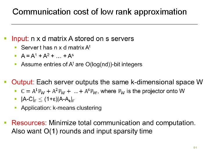
Communication cost of low rank approximation 81

Work on Distributed Low Rank Approximation § [FSS]: First protocol for the row-partition model. § O(sdk/ε) real numbers of communication § Don’t analyze bit complexity (can be large) § SVD Running time, see also [BKLW] § [KVW]: O(skd/ε) communication in arbitrary partition model § [BWZ]: O(skd) + poly(sk/ε) words of communication in arbitrary partition model. Input sparsity time § Matching Ω(skd) words of communication lower bound § Variants: kernel low rank approximation [BLSWX], low rank approximation of an implicit matrix [WZ], sparsity [BWZ] 82

Outline of Distributed Protocols § [FSS] protocol § [KVW] protocol § [BWZ] protocol 83

Constructing a Coreset [FSS] § 84

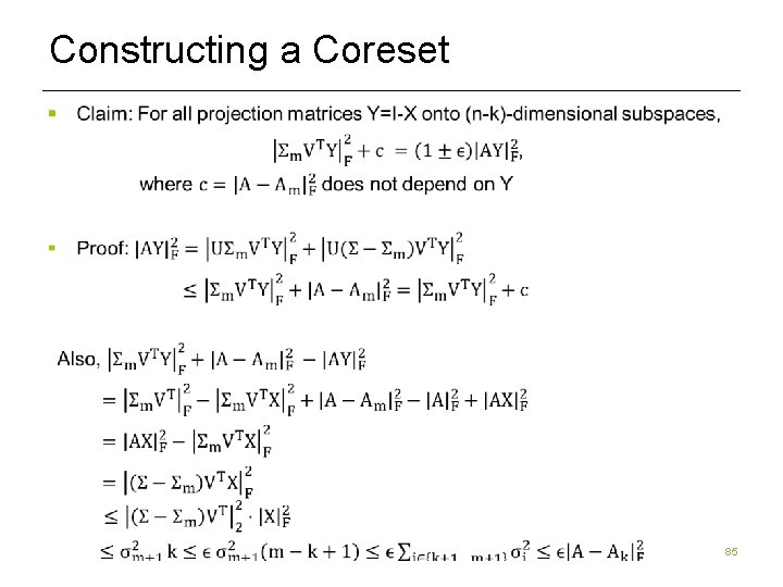
Constructing a Coreset § 85

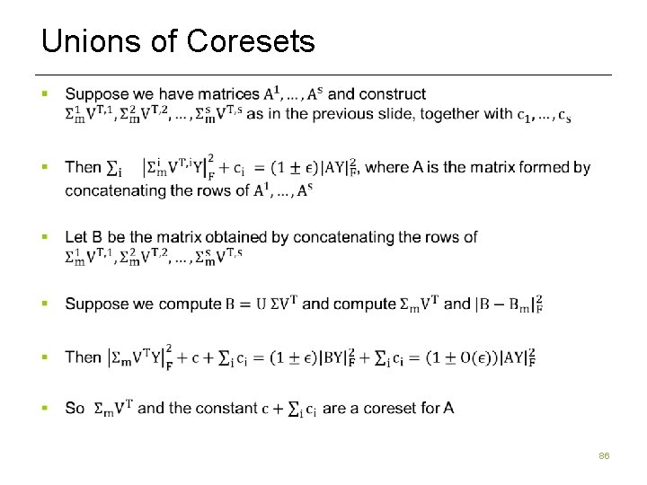
Unions of Coresets § 86

[FSS] Row-Partition Protocol [KVW] protocol will handle 2, 3, Problems: Coordinator and 4 1. sdk/ε real numbers of communication 2. bit complexity can be large 3. running time for SVDs [BLKW] 4. doesn’t work in arbitrary partition model … This is an SVD-based protocol. Maybe our random matrix techniques can improve communication just like they improved computation? 87

[KVW] Arbitrary Partition Model Protocol § Inspired by the sketching algorithm presented earlier Problems: § Let S be one of the k/ε x n random matrices discussed § Can’t output projection of At onto SA since § S can be generated pseudorandomly from small seed the rank is too large § Coordinator sends small seed for S to all servers § Could communicate this projection to the t and sends it to Coordinator § Server t computes SA coordinator who could find a k-dimensional space, but communication depends on n § Coordinator sends Σt=1 s SAt = SA to all servers § There is a good k-dimensional subspace inside of SA. If we knew it, t-th server could output projection of At onto it 88

[KVW] protocol § Phase 1: § Learn the row space of SA optimal k-dimensional space in SA SA cost · (1+ε)|A-Ak|F 89

[KVW] protocol § Phase 2: § Find an approximately optimal space W inside of SA optimal space in SA approximate space W in SA SA cost · (1+ε)2|A-Ak|F 90

[BWZ] Protocol § 91

[BWZ] Protocol § Intuitively, U looks like top k left singular vectors of SA Top k right singular vectors of SA work because S is a projectioncost preserving sketch! 92

[BWZ] Analysis § 93

Conclusions for Distributed Low Rank Approximation § [BWZ] Optimal O(sdk) + poly(sk/ε) communication protocol for low rank approximation in arbitrary partition model § Handle bit complexity by adding Tao/Vu noise § Input sparsity time § 2 rounds, which is optimal [W] § Optimal data stream algorithms improves [CW, L, GP] § Communication of other optimization problems? § Computing the rank of an n x n matrix over the reals § Linear Programming § Graph problems: Matching § etc. 94

Additional Time-Permitting Topics § Will cover some recent topics at a research-level (many details omitted) § Weighted Low Rank Approximation § Regression and Low Rank Approximation with MEstimator Loss Functions § Finding Heavy Hitters in a Data Stream optimally 95