Skadu Efficient Vector Shadow Memories for PolyScopic Program

Skadu: Efficient Vector Shadow Memories for Poly-Scopic Program Analysis Donghwan Jeon*, Saturnino Garcia+, and Michael Bedford Taylor UC San Diego * Now at Google, Inc. + Now at University of San Diego Skadu means ‘Shadow’ in Afrikaans. 1

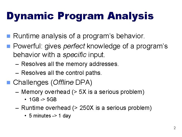
Dynamic Program Analysis Runtime analysis of a program’s behavior. n Powerful: gives perfect knowledge of a program’s behavior with a specific input. n – Resolves all the memory addresses. – Resolves all the control paths. n Challenges (Offline DPA) – Memory overhead (> 5 X is a serious problem) • 1 GB -> 5 GB – Runtime overhead (> 250 X is a serious problem) • 5 minutes -> 1 day 2

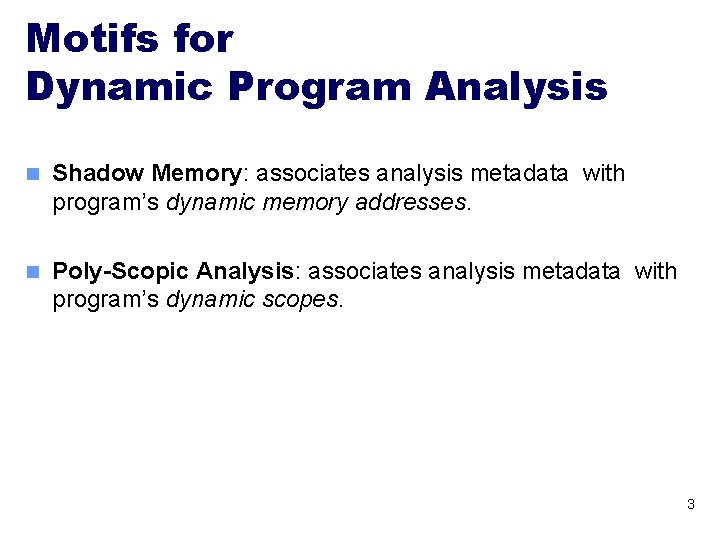
Motifs for Dynamic Program Analysis n Shadow Memory: associates analysis metadata with program’s dynamic memory addresses. n Poly-Scopic Analysis: associates analysis metadata with program’s dynamic scopes. 3

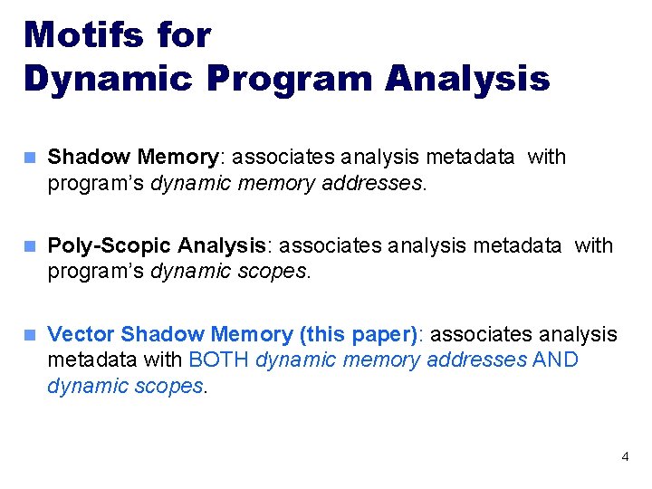
Motifs for Dynamic Program Analysis n Shadow Memory: associates analysis metadata with program’s dynamic memory addresses. n Poly-Scopic Analysis: associates analysis metadata with program’s dynamic scopes. n Vector Shadow Memory (this paper): associates analysis metadata with BOTH dynamic memory addresses AND dynamic scopes. 4

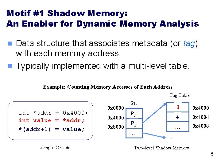
Motif #1 Shadow Memory: An Enabler for Dynamic Memory Analysis Data structure that associates metadata (or tag) with each memory address. n Typically implemented with a multi-level table. n Example: Counting Memory Accesses of Each Address Tag Table int *addr = 0 x 4000; int value = *addr; *(addr+1) = value; Sample C Code 0 x 0000 0 x 4000 0 x 8000 Ptr 01 P 0 0 x 4000 43 0 x 4004 PP 11 … 0 x 4008 … … Two-level Shadow Memory 5

Dynamic Program Analyses Employing Shadow Memory n n n Critical Path Analysis [1988] – Finds the longest dynamic dependence chain in a program. – Employs shadow memory to propagate earliest completion time of memory operations. – Useful for approximating the quantity of parallelism available in a program. Taint. Check [2005] Valgrind [2007] Dr. Memory [2011] … 6

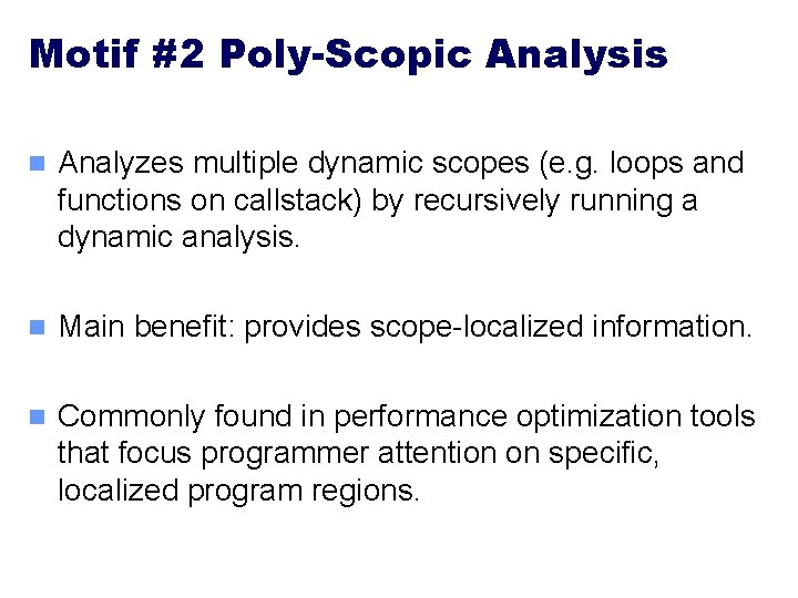
Motif #2 Poly-Scopic Analysis n Analyzes multiple dynamic scopes (e. g. loops and functions on callstack) by recursively running a dynamic analysis. n Main benefit: provides scope-localized information. n Commonly found in performance optimization tools that focus programmer attention on specific, localized program regions.

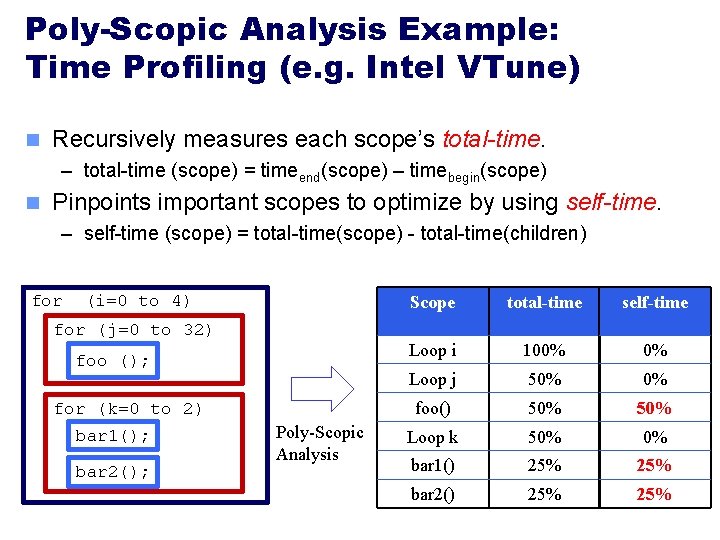
Poly-Scopic Analysis Example: Time Profiling (e. g. Intel VTune) n Recursively measures each scope’s total-time. – total-time (scope) = timeend(scope) – timebegin(scope) n Pinpoints important scopes to optimize by using self-time. – self-time (scope) = total-time(scope) - total-time(children) for (i=0 to 4) for (j=0 to 32) foo (); for (k=0 to 2) bar 1(); bar 2(); Poly-Scopic Analysis Scope total-time self-time Loop i 100% 0% Loop j 50% 0% foo() 50% Loop k 50% 0% bar 1() 25% bar 2() 25%

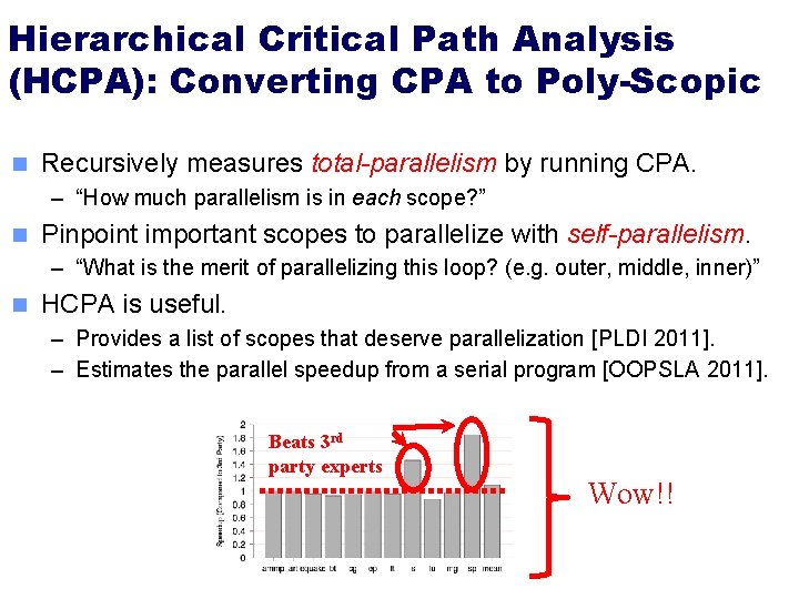
Hierarchical Critical Path Analysis (HCPA): Converting CPA to Poly-Scopic n Recursively measures total-parallelism by running CPA. – “How much parallelism is in each scope? ” n Pinpoint important scopes to parallelize with self-parallelism. – “What is the merit of parallelizing this loop? (e. g. outer, middle, inner)” n HCPA is useful. – Provides a list of scopes that deserve parallelization [PLDI 2011]. – Estimates the parallel speedup from a serial program [OOPSLA 2011]. Beats 3 rd party experts Wow!!

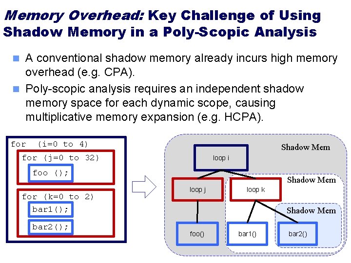
Memory Overhead: Key Challenge of Using Shadow Memory in a Poly-Scopic Analysis A conventional shadow memory already incurs high memory overhead (e. g. CPA). n Poly-scopic analysis requires an independent shadow memory space for each dynamic scope, causing multiplicative memory expansion (e. g. HCPA). n for (i=0 to 4) Shadow Mem for (j=0 to 32) loop i foo (); for (k=0 to 2) bar 1(); bar 2(); Shadow Mem loop j loop k Shadow Mem foo() bar 1() bar 2()

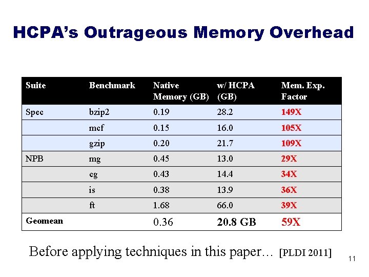
HCPA’s Outrageous Memory Overhead Suite Benchmark Native w/ HCPA Memory (GB) Mem. Exp. Factor Spec bzip 2 0. 19 28. 2 149 X mcf 0. 15 16. 0 105 X gzip 0. 20 21. 7 109 X mg 0. 45 13. 0 29 X cg 0. 43 14. 4 34 X is 0. 38 13. 9 36 X ft 1. 68 66. 0 39 X 0. 36 20. 8 GB 59 X NPB Geomean Before applying techniques in this paper… [PLDI 2011] 11

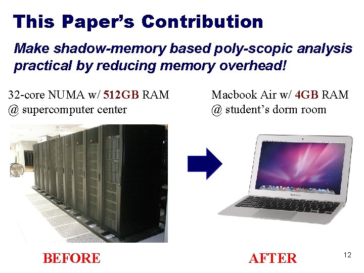
This Paper’s Contribution Make shadow-memory based poly-scopic analysis practical by reducing memory overhead! 32 -core NUMA w/ 512 GB RAM @ supercomputer center BEFORE Macbook Air w/ 4 GB RAM @ student’s dorm room AFTER 12

Outline n n n Introduction Vector Shadow Memory Lightweight Tag Validation Efficient Storage Management Experimental Results Conclusion 13

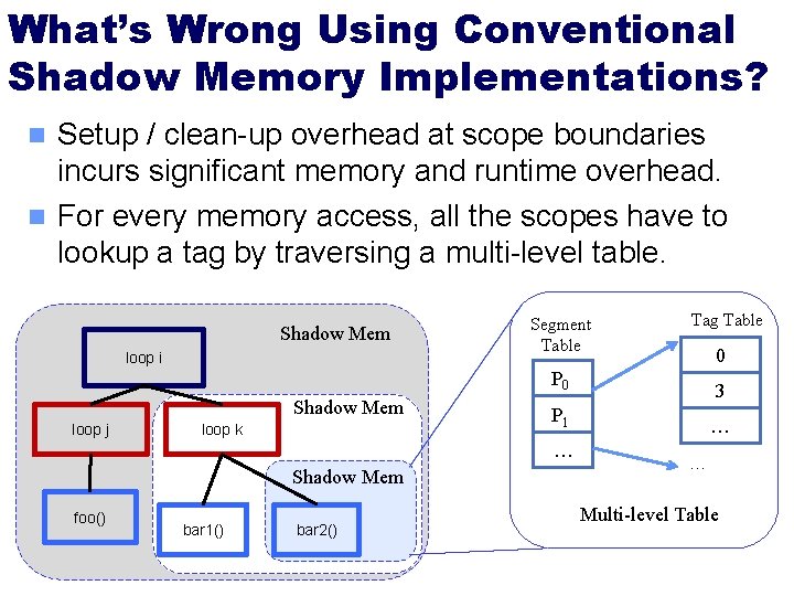
What’s Wrong Using Conventional Shadow Memory Implementations? Setup / clean-up overhead at scope boundaries incurs significant memory and runtime overhead. n For every memory access, all the scopes have to lookup a tag by traversing a multi-level table. n Shadow Mem loop i Shadow Mem loop j loop k Segment Table foo() bar 1() bar 2() 0 P 0 3 P 1 … … Shadow Mem Tag Table … Multi-level Table

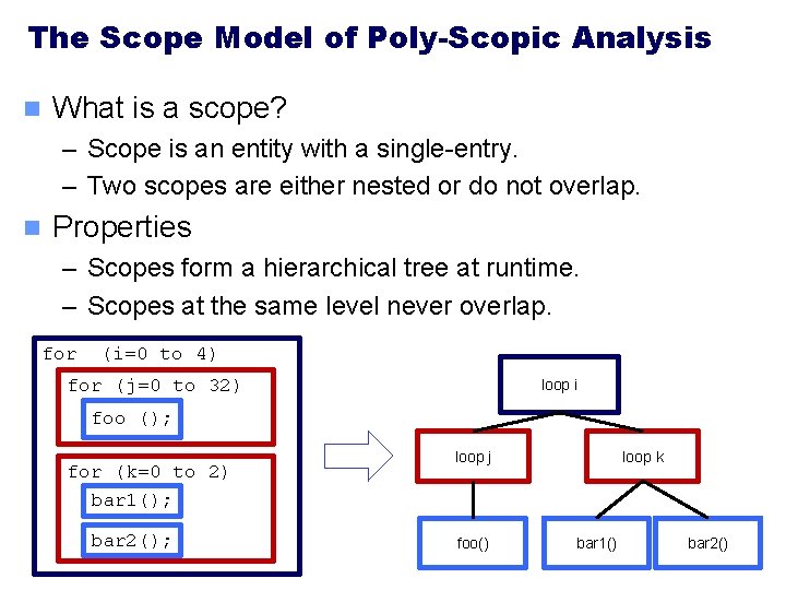
The Scope Model of Poly-Scopic Analysis n What is a scope? – Scope is an entity with a single-entry. – Two scopes are either nested or do not overlap. n Properties – Scopes form a hierarchical tree at runtime. – Scopes at the same level never overlap. for (i=0 to 4) for (j=0 to 32) loop i foo (); for (k=0 to 2) bar 1(); bar 2(); loop j foo() loop k bar 1() bar 2()

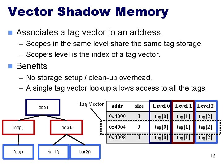
Vector Shadow Memory n Associates a tag vector to an address. – Scopes in the same level share the same tag storage. – Scope’s level is the index of a tag vector. n Benefits – No storage setup / clean-up overhead. – A single tag vector lookup allows access to all the tags. Tag Vector loop i loop j foo() loop k bar 1() bar 2() addr size Level 0 Level 1 Level 2 0 x 4000 3 tag[0] tag[1] tag[2] 0 x 4004 3 tag[0] tag[1] tag[2] 0 x 4008 3 tag[0] tag[1] tag[2] 16

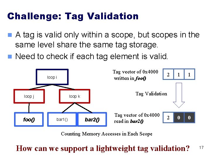
Challenge: Tag Validation A tag is valid only within a scope, but scopes in the same level share the same tag storage. n Need to check if each tag element is valid. n Tag vector of 0 x 4000 written in foo() loop i loop j foo() 1 1 0 0 Tag Validation loop k bar 1() 2 bar 2() Tag vector of 0 x 4000 read in bar 2() 2 Counting Memory Accesses in Each Scope How can we support a lightweight tag validation? 17

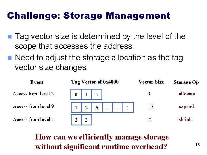
Challenge: Storage Management Tag vector size is determined by the level of the scope that accesses the address. n Need to adjust the storage allocation as the tag vector size changes. n Event Vector Size Tag Vector of 0 x 4000 Access from level 2 0 1 5 Access from level 9 1 2 6 Access from level 1 2 3 … … 1 Storage Op 3 allocate 10 expand 2 shrink How can we efficiently manage storage without significant runtime overhead? 18

Outline n n n Introduction Vector Shadow Memory Lightweight Tag Validation Efficient Storage Management Experimental Results Conclusion 19

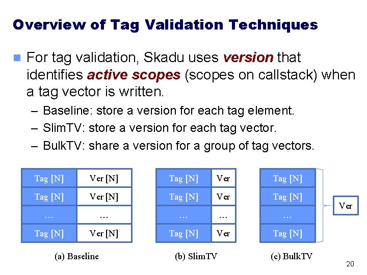
Overview of Tag Validation Techniques n For tag validation, Skadu uses version that identifies active scopes (scopes on callstack) when a tag vector is written. – Baseline: store a version for each tag element. – Slim. TV: store a version for each tag vector. – Bulk. TV: share a version for a group of tag vectors. Tag [N] Ver [N] Tag [N] Ver Tag [N] … … … Tag [N] Ver [N] Tag [N] Ver Tag [N] (a) Baseline (b) Slim. TV (c) Bulk. TV Ver 20

Baseline Tag Validation n for each level If (Ver [level] != Ver_active[level]) { // invalidate the level Tag[level] Init_Val Ver[level] Ver_active[level] ); } Tag [N] Ver [N] … … Tag [N] Ver [N] (a) Baseline 21

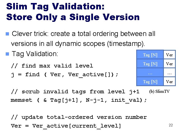
Slim Tag Validation: Store Only a Single Version Clever trick: create a total ordering between all versions in all dynamic scopes (timestamp). n Tag Validation: Tag [N] Ver … … Tag [N] Ver n // find max valid level j = find ( Ver, Ver_active[]); // scrub invalid tags from level j+1 memset ( & Tag[j+1], N-j-1, init_val); // update total-ordered version number Ver = Ver_active[current_level] (b) Slim. TV 22

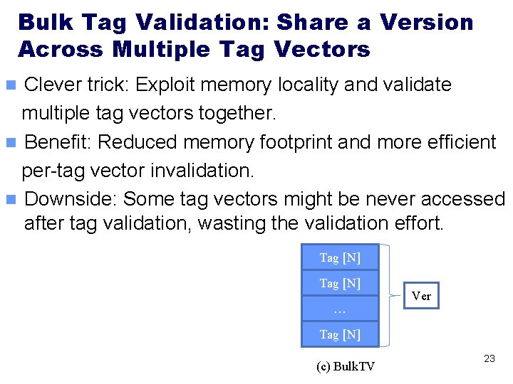
Bulk Tag Validation: Share a Version Across Multiple Tag Vectors Clever trick: Exploit memory locality and validate multiple tag vectors together. n Benefit: Reduced memory footprint and more efficient per-tag vector invalidation. n Downside: Some tag vectors might be never accessed after tag validation, wasting the validation effort. n Tag [N] … Ver Tag [N] (c) Bulk. TV 23

Outline n n n Introduction Vector Shadow Memory Lightweight Tag Validation Efficient Storage Management Experimental Results Conclusion 24

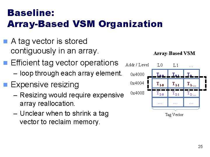
Baseline: Array-Based VSM Organization A tag vector is stored contiguously in an array. n Efficient tag vector operations n – loop through each array element. n Expensive resizing – Resizing would require expensive array reallocation. – Unclear when to shrink a tag vector to reclaim memory. Array-Based VSM Addr / Level L 0 L 1 … 0 x 4000 T 0 -1 T 0 -… 0 x 4004 T 1 -0 T 1 -1 T 1 -… 0 x 4008 T 2 -0 T 2 -1 T 2 -… … Tag Vector 25

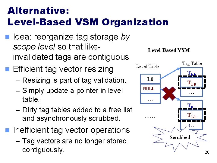
Alternative: Level-Based VSM Organization Idea: reorganize tag storage by scope level so that likeinvalidated tags are contiguous n Efficient tag vector resizing n – Resizing is part of tag validation. – Simply update a pointer in level table. – Dirty tag tables added to a free list and asynchronously scrubbed. n Inefficient tag vector operations – Tag vectors are no longer stored contiguously. Level-Based VSM Level Table L 0 NULL L 1 Tag Table T 0 -0 T 1 -0 … … T 0 -1 …… T 1 -1 … Scrubbed 26

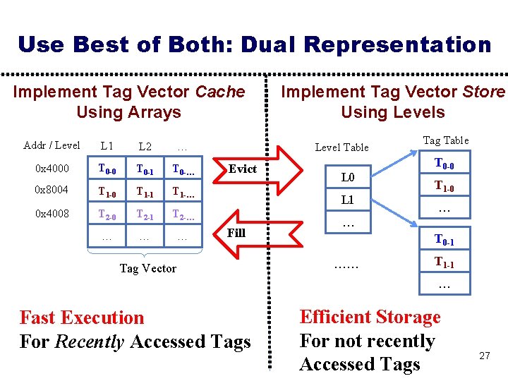
Use Best of Both: Dual Representation Implement Tag Vector Cache Using Arrays Addr / Level L 1 L 2 … 0 x 4000 T 0 -1 T 0 -… 0 x 8004 T 1 -0 T 1 -1 T 1 -… 0 x 4008 T 2 -0 T 2 -1 T 2 -… … Implement Tag Vector Store Using Levels Level Table Evict L 0 L 1 Fill Tag Vector Tag Table T 0 -0 T 1 -0 … … T 0 -1 …… T 1 -1 … Fast Execution For Recently Accessed Tags Efficient Storage For not recently Accessed Tags 27

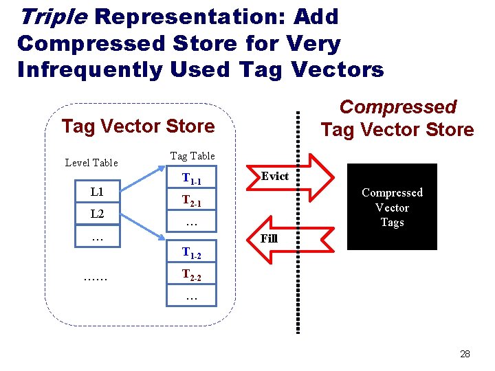
Triple Representation: Add Compressed Store for Very Infrequently Used Tag Vectors Compressed Tag Vector Store Level Table L 1 L 2 Tag Table T 1 -1 Compressed Vector Tags T 2 -1 … … T 1 -2 …… Evict Fill T 2 -2 … 28

Outline n n n Introduction Vector Shadow Memory Lightweight Tag Validation Efficient Storage Management Experimental Results Conclusion 29

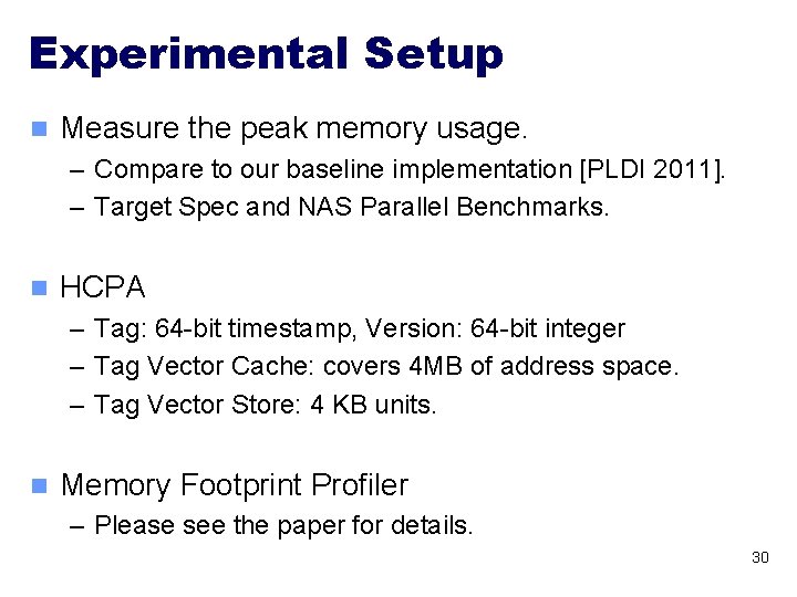
Experimental Setup n Measure the peak memory usage. – Compare to our baseline implementation [PLDI 2011]. – Target Spec and NAS Parallel Benchmarks. n HCPA – Tag: 64 -bit timestamp, Version: 64 -bit integer – Tag Vector Cache: covers 4 MB of address space. – Tag Vector Store: 4 KB units. n Memory Footprint Profiler – Please see the paper for details. 30

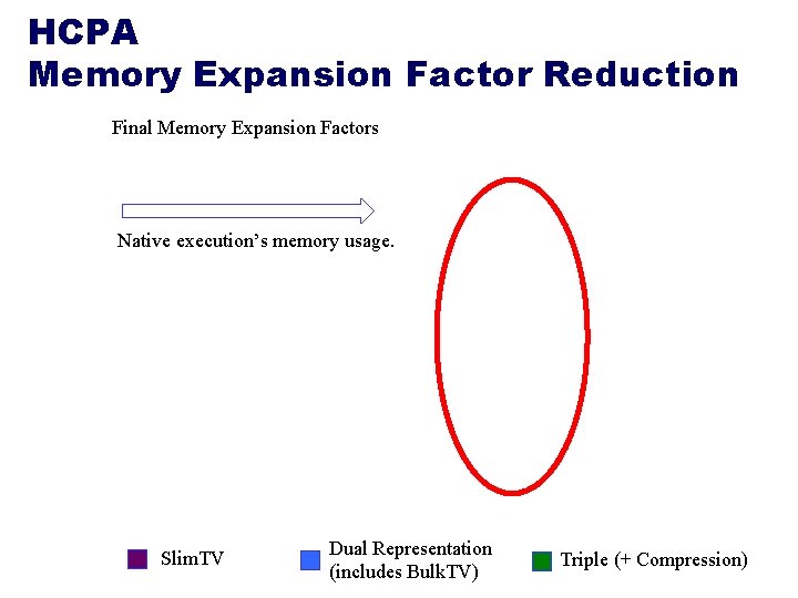
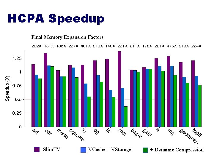
HCPA Memory Expansion Factor Reduction Final Memory Expansion Factors Native execution’s memory usage. Slim. TV Dual Representation (includes Bulk. TV) Triple (+ Compression)

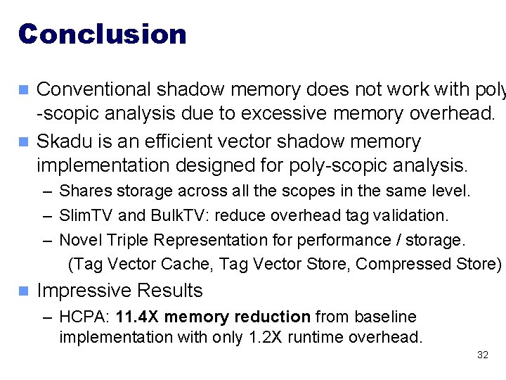
Conclusion Conventional shadow memory does not work with poly -scopic analysis due to excessive memory overhead. n Skadu is an efficient vector shadow memory implementation designed for poly-scopic analysis. n – Shares storage across all the scopes in the same level. – Slim. TV and Bulk. TV: reduce overhead tag validation. – Novel Triple Representation for performance / storage. (Tag Vector Cache, Tag Vector Store, Compressed Store) n Impressive Results – HCPA: 11. 4 X memory reduction from baseline implementation with only 1. 2 X runtime overhead. 32

HCPA Speedup Final Memory Expansion Factors Slim. TV VCache + VStorage + Dynamic Compression