SIR and SIRS Models Cindy Wu Hyesu Kim

SIR and SIRS Models Cindy Wu, Hyesu Kim, Michelle Zajac, Amanda Clemm SPWM 2011

Our group! � Cindy Wu � Gonzaga University � Dr. Burke � Hyesu Kim � Manhattan College � Dr. Tyler � Michelle Zajac � Alfred University � Dr. Petrillo � Amanda Clemm � Scripps College � Dr. Ou

Cindy Wu � Why Math? � Friends � Coolest thing you learned � Number Theory � Why SPWM? � DC>Spokane � Otherwise, unproductive

Hyesu Kim � Why math? ◦ Common language ◦ Challenging � Coolest learned thing you ◦ Math is everywhere ◦ Anything is possible � Why SPWM? ◦ Work or grad school? ◦ Possible careers

Michelle Zajac � Why math? ◦ Interesting ◦ Challenging � Coolest Learned Thing you ◦ RSA Cryptosystem � Why SPWM? ◦ Grad school ◦ Learn something new

Amanda Clemm � Why Math? ◦ Applications ◦ Challenge � Coolest Learned Thing you ◦ Infinitude of the primes � Why SPWM? ◦ Life after college ◦ DC

Epidemiology � Study of disease occurrence � Actual experiments vs Models � Prevention and control procedures

Epidemic vs Endemic � Epidemic: Unusually large, short term outbreak of a disease � Endemic: The disease persists � Vital Dynamics: Births and natural deaths accounted for � Vital Dynamics play a bigger part in an endemic

Populations � Total population=N ( a constant) � Population fractions ◦ S(t)=susceptible pop. fraction ◦ I(t)=infected pop. fraction ◦ R(t)=removed pop. fraction

SIR vs SIRS Model � Both are epidemiological models that compute the number of people infected with a contagious illness in a population over time � SIR: Those infected that recover gain permanent immunity (ODE) � SIRS: Those infected that recover gain temporary immunity (DDE) � NOTE: Person to person contact only

PART ONE: SIR Models using ODES

Variables and Values of Importance � λ=daily contact rate ◦ Homogeneously mixing ◦ Does not change seasonally �γ =daily recovery removal rate � σ=λ/ γ ◦ The contact number

The SIR Model without Vital Dynamics � Model for infection that confers permanent immunity � Compartmental diagram λSNI NS Susceptibles � (NS(t))’=-λSNI � (NI(t))’= NI Infectives λSNI- γNI � (NR(t))’= γNI ϒNI NR Removeds S’(t)=-λSI I’(t)=λSI-ϒI

Theorem � S’(t)=-λSI � I’(t)=λSI-ϒI � Let S(t) and I(t) be solutions of this system. � CASE ONE: σS₀≤ 1 ◦ I(t) decreases to 0 as t goes to infinity (no epidemic) � CASE TWO: σS₀>1 ◦ I(t) increases up to a maximum of: 1 -R₀-1/σ-ln(σS₀)/σ Then it decreases to 0 as t goes to infinity (epidemic) σS₀=(S₀λ)/ϒ Initial Susceptible population fraction Daily contact rate Daily recovery removal rate

MATLAB Epidemic

PART TWO: SIRS Models using DDES

Equations and Variables � d. S/dt=μ[1 -S(t)]-ΒI(t)S(t)+r γ γ � d. I/dt=ΒI(t)S(t)-(μ+γ)I(t) e-μτI(t-τ) � d. R/dt=γI(t)-μR(t)-rγγe-μτI(t-τ) � μ=death rate � Β=transmission coefficient � γ=recovery rate � τ=amount of time before re-susceptibility � e-μτ=fraction who recover at time t-τ who survive to time t � rγ=fraction of pop. that become re-susceptible

Equilibrium Solutions � Focus on the endemic steady state (R 0 S=1) Reproductive number: R 0=Β/(μ+γ) � Sc=1/R 0 � Ic=[(μ/Β)(ℛ 0 -1)]/[1 -(rγγ)(e-μτ )/(μ+γ)] Our goal is now to determine stability

Rescaled Equations � dx/dt=-y-εx(a+by)+ry(t-τ) � dy/dt=x(1+y) where ε=√(μΒ)/γ 2<<1 and r=(e-μτ rγγ)/(μ+γ) and a, b are really close to 1 � Rescaled equation for r is a primary control parameter � r is the fraction of those in S who return to S after being infected

More about r � r=(e-μτ rγγ)/(μ+γ) � What � Thus, � So does rγ=1 mean? r max=γ e-μτ /(μ+γ) we have: 0≤r≤ r max<1

Characteristic Equation � λ 2+εaλ+1 -re-λτ=0 � Note: When r=0, the delay term is removed leaving a scaled SIR model such that the endemic steady state is stable for R 0>1

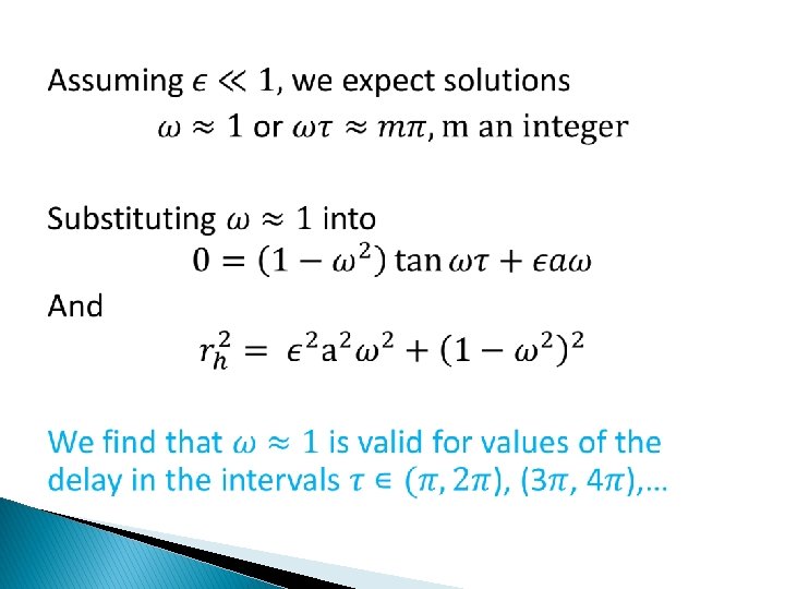
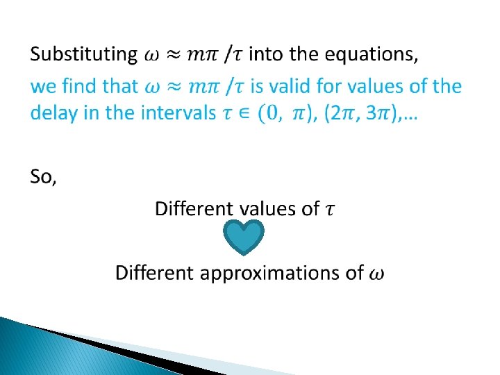
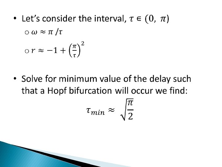
When does the Hopf bifurcation occur?

In terms of the original variables…

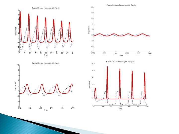
r=0. 005

r=0. 005 (Zoomed in)

r=0. 02

r=0. 02 (Zoomed in)

r=0. 03

r=0. 03 (Zoomed in)

r=0. 9

Conclusion � In our ODE we represented an epidemic � DDE case more accurately represents longer term population behavior � Changing the delay and resusceptible value changes the models behavior � Better prevention and control strategies