Singular Value Decomposition and the Conjugate Gradient Method

Singular Value Decomposition and the Conjugate Gradient Method CSE 5400 Joy Moore

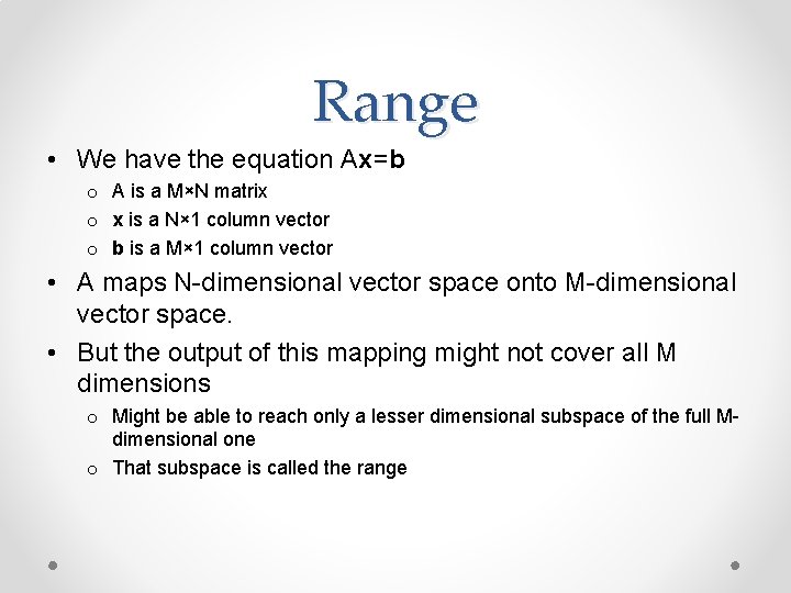
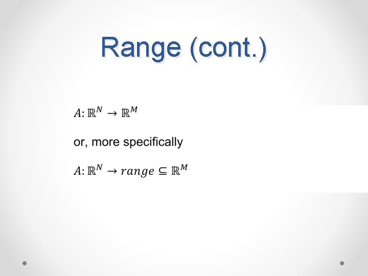
Range • We have the equation Ax=b o A is a M×N matrix o x is a N× 1 column vector o b is a M× 1 column vector • A maps N-dimensional vector space onto M-dimensional vector space. • But the output of this mapping might not cover all M dimensions o Might be able to reach only a lesser dimensional subspace of the full Mdimensional one o That subspace is called the range

Range (cont. )

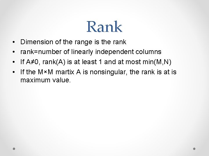
Rank • • Dimension of the range is the rank=number of linearly independent columns If A≠ 0, rank(A) is at least 1 and at most min(M, N) If the M×M martix A is nonsingular, the rank is at is maximum value.

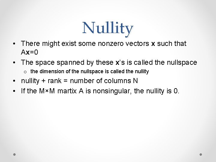
Nullity • There might exist some nonzero vectors x such that Ax=0 • The space spanned by these x’s is called the nullspace o the dimension of the nullspace is called the nullity • nullity + rank = number of columns N • If the M×M martix A is nonsingular, the nullity is 0.

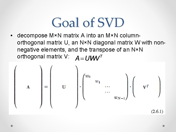
Goal of SVD • decompose M×N matrix A into an M×N columnorthogonal matrix U, an N×N diagonal matrix W with nonnegative elements, and the transpose of an N×N orthogonal matrix V:

Columns of U • Orthonormal set of basis vectors that span the range • Any element in the range can be written as a linear combination of U’s columns. • If the constant vector b is in the range of A, then the equation Ax=b has a unique solution x. o If not, we can use the least squares solution

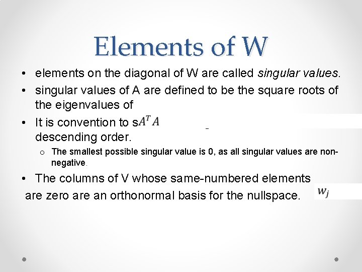
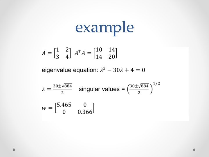
Elements of W • elements on the diagonal of W are called singular values. • singular values of A are defined to be the square roots of the eigenvalues of • It is convention to sort these singular values in descending order. o The smallest possible singular value is 0, as all singular values are nonnegative. • The columns of V whose same-numbered elements are zero are an orthonormal basis for the nullspace.

example

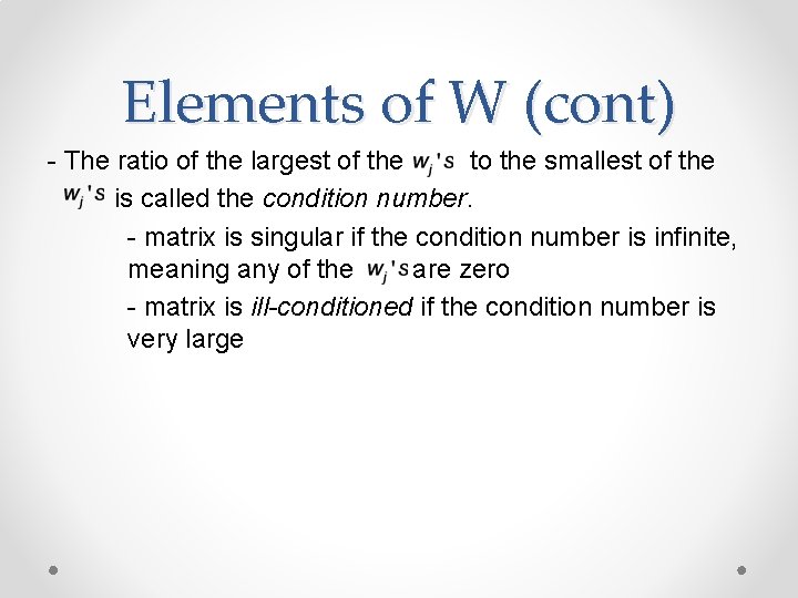
Elements of W (cont) - The ratio of the largest of the to the smallest of the is called the condition number. - matrix is singular if the condition number is infinite, meaning any of the are zero - matrix is ill-conditioned if the condition number is very large

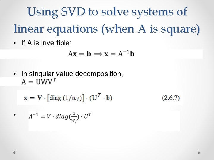
Using SVD to solve systems of linear equations (when A is square) • If A is invertible: • In singular value decomposition, •

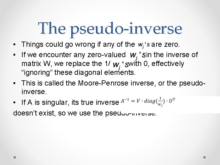
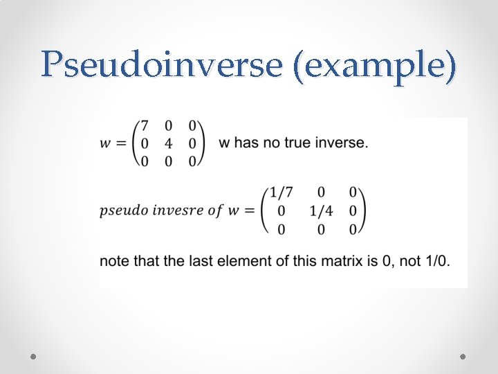
The pseudo-inverse • Things could go wrong if any of the are zero. • If we encounter any zero-valued in the inverse of matrix W, we replace the 1/ with 0, effectively “ignoring” these diagonal elements. • This is called the Moore-Penrose inverse, or the pseudoinverse. • If A is singular, its true inverse doesn’t exist, so we use the pseudo-inverse.

Pseudoinverse (example)

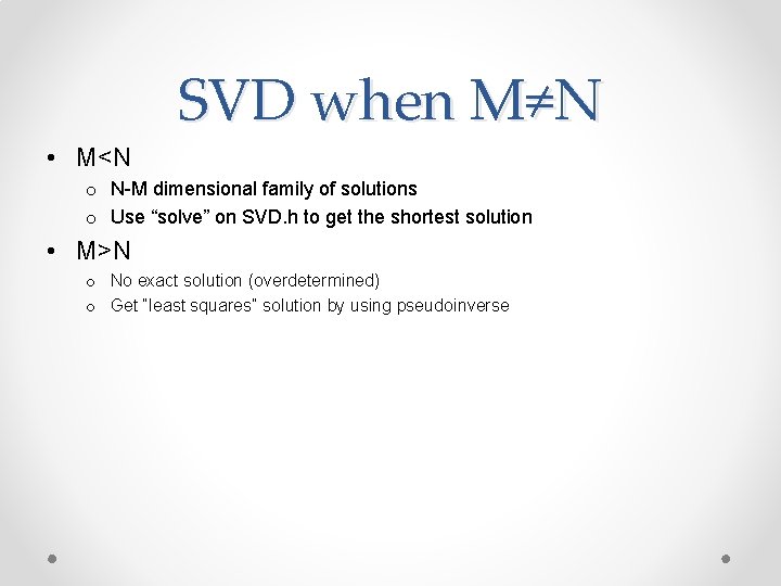
SVD when M≠N • M<N o N-M dimensional family of solutions o Use “solve” on SVD. h to get the shortest solution • M>N o No exact solution (overdetermined) o Get “least squares” solution by using pseudoinverse

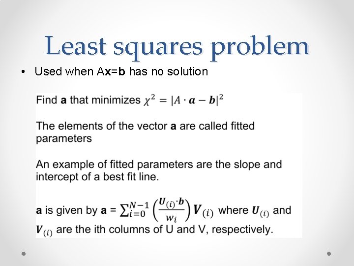
Least squares problem • Used when Ax=b has no solution

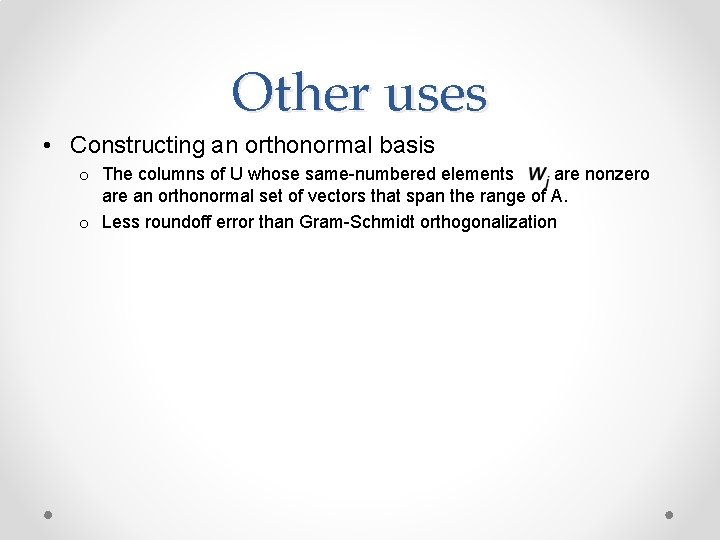
Other uses • Constructing an orthonormal basis o The columns of U whose same-numbered elements are nonzero are an orthonormal set of vectors that span the range of A. o Less roundoff error than Gram-Schmidt orthogonalization

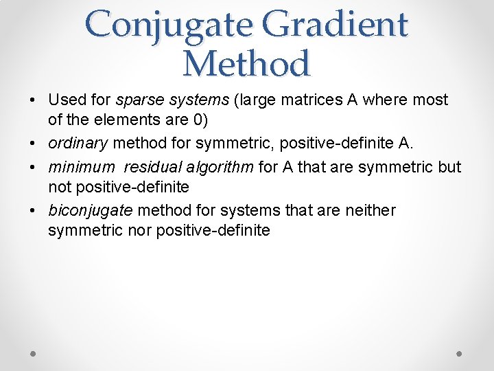
Conjugate Gradient Method • Used for sparse systems (large matrices A where most of the elements are 0) • ordinary method for symmetric, positive-definite A. • minimum residual algorithm for A that are symmetric but not positive-definite • biconjugate method for systems that are neither symmetric nor positive-definite

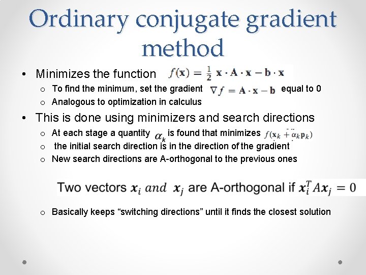
Ordinary conjugate gradient method • Minimizes the function o To find the minimum, set the gradient o Analogous to optimization in calculus equal to 0 • This is done using minimizers and search directions o At each stage a quantity is found that minimizes o the initial search direction is in the direction of the gradient o New search directions are A-orthogonal to the previous ones o Basically keeps “switching directions” until it finds the closest solution

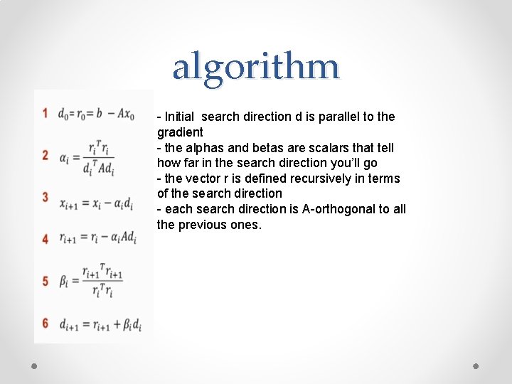
algorithm - Initial search direction d is parallel to the gradient - the alphas and betas are scalars that tell how far in the search direction you’ll go - the vector r is defined recursively in terms of the search direction - each search direction is A-orthogonal to all the previous ones.

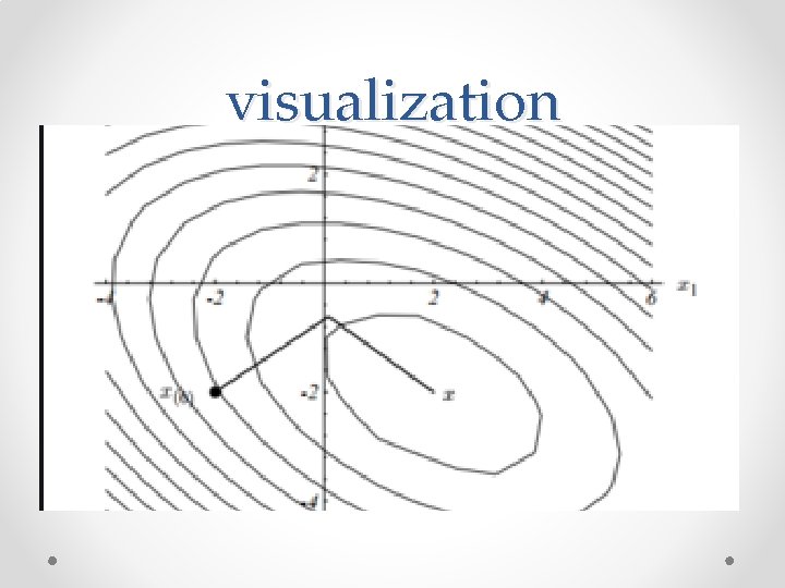
visualization

references • Press, William H. , and William T. Vetterling. Numerical Recipes. Cambridge Univ. Press, 2007. • “Conjugate Gradient Method. ” Wikipedia, Wikimedia Foundation, 21 May 2019, https: //en. wikipedia. org/wiki/Conjugate_gradient_method. • https: //www. youtube. com/watch? v=e. AYoh. MUp. PMA