Single Source Shortest Path and Linear Programming Dr

Single Source Shortest Path and Linear Programming Dr. Mustafa Sakalli Marmara Univ. Mid May of 2009, CS 246

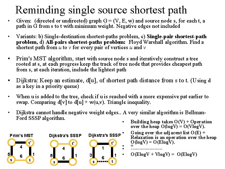
Reminding single source shortest path • Given: (directed or undirected) graph G = (V, E, w) and source node s, for each t, a path in G from s to t with minimum weight. Negative edges not included • Variants: b) Single-destination shortest-paths problem, c) Single-pair shortest-path problem, d) All-pairs shortest-paths problem: Floyd Warshall algorithm. Find a shortest path from u to v for every pair of vertices u and v • Prim's MST algorithm, start with source node s and iteratively construct a tree rooted at s, at each progress keep the track of tree node that provides cheapest path from s, at each iteration, include the lightest path • Dijkstra: Keep an estimate, d[u], of shortest path distance from s to t. (Using d as a key in a priority queue) • When u is added to the tree, check if u is reached with a more expensive pat earlier to swap. Comparing d[v] to d[u] + w(u, v). Triangle inequality. • Dijkstra cannot handle negative weight edges. . A very similar algorithm is Bellman. Ford SSSP algorithm. • Prim's MST 4 5 s 6 Dijkstra's SSSP t’ 4 1 t 5 s 6 Dijkstra's SSSP t’ 1 1 3 s 6 t’ 1 t • • Building heap takes O(V) + Operation over the heap O(log. V) = O(Vlog. V). Going over the adjacent list O(E) + Relaxation is an operation over the heap O(log. V) = O(Elog. V). + ---------- O(Elog. V + Vlog. V) = O(Elog. V)

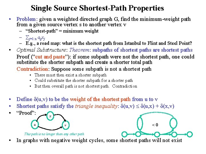
Single Source Shortest-Path Properties • Problem: given a weighted directed graph G, find the minimum-weight path from a given source vertex s to another vertex v – – – “Shortest-path” = minimum weight j=1: n aijxj E. g. , a road map: what is the shortest path from Istanbul to Flint and Steel Point? • Optimal Substructure: Theorem: subpaths of shortest paths are shortest paths Proof (”cut and paste”): if some subpath were not the shortest path, one could substitute the shorter subpath and create a shorter total path Contradiction: Suppose some subpath is not a shortest path : Suppose • There must then exist a shorter subpath • Could substitute the shorter subpath for a shorter path • But then overall path is not shortest path. Contradiction • Define (u, v) to be the weight of the shortest path from u to v • Shortest paths satisfy the triangle inequality: (u, v) (u, x) + (x, v) • “Proof”: x u v <0 This path is no longer than any other path • In graphs with negative weight cycles, some shortest paths will not exist

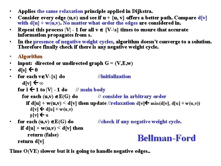
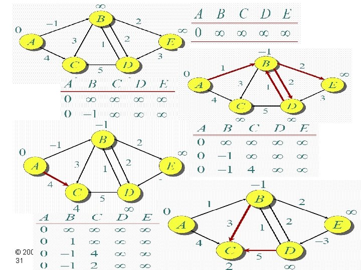
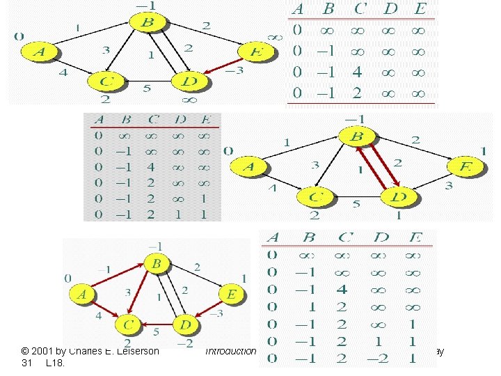
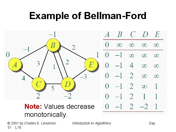
• • Applies the same relaxation principle applied in Dijkstra. Consider every edge (u, v) and see if u + {u, v} offers a better path. Compare d[v] with d[u] + w(u, v). No matter what order the edges are considered in. Repeat this process |V| - 1 for all v {V-s} times to ensure that accurate information propagates from s. In the presence of negative weight cycles, algorithm doesn’t converge to a solution. Therefore finally check if there is any negative weight cycle. Algorithm input: directed or undirected graph G = (V, E, w) d[s] 0 for each v V-{s} do //initialization d[v] ∞ for i 1 to |V| - 1 do // main body for each (u, v) E(G) do // consider in arbitrary order if d[u] + w(u, v) < d[v] then update //relaxation d[v] min(d[v], d[u] + w(u, v)) d[v] d[u] + w(u, v) p[v] u • for each (u, v) E(G) do if d[u] + w(u, v) < d[v] then return (false) return d[v] //check if any negative weight cycle. Bellman-Ford Time O(VE) slower but it is going to handle negative edges. .

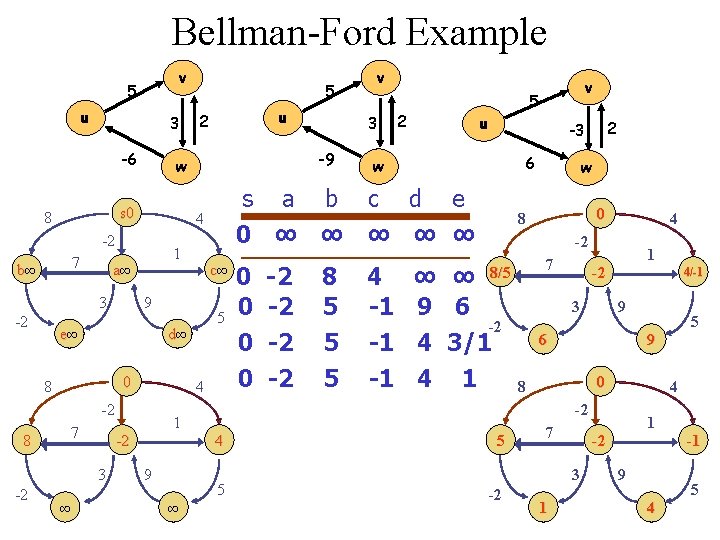
Bellman-Ford Example v 5 u 3 -6 7 3 -2 1 a∞ 0 8 4 -2 7 8 ∞ 1 -2 3 -2 5 d∞ 9 ∞ 2 0 0 -2 -2 8 5 5 5 u 2 -3 6 w 4 -1 -1 -1 v 5 s a b c d e 0 ∞ ∞ ∞ c∞ 9 e∞ 3 -9 4 -2 b∞ u 2 w s 0 8 5 v w 0 8 4 -2 ∞ ∞ 8/5 9 6 -2 4 3/1 4 1 8 7 1 -2 3 4/-1 9 6 9 0 4 -2 4 5 5 7 1 1 -2 3 -2 5 9 4 -1 5

© 2001 by Charles E. Leiserson 31 L 18. Introduction to Algorithms Day

© 2001 by Charles E. Leiserson 31 L 18. Introduction to Algorithms Day

Example of Bellman-Ford Note: Values decrease monotonically. © 2001 by Charles E. Leiserson 31 L 18. Introduction to Algorithms Day

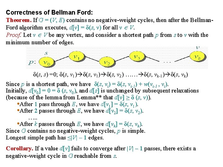
Correctness of Bellman Ford: Theorem. If G = (V, E) contains no negative-weight cycles, then after the Bellman. Ford algorithm executes, d[v] = (s, v) for all v V. Proof. Let v V be any vertex, and consider a shortest path p from s to v with the minimum number of edges. δ(s, s) =0; δ(s, v 1) δ(s, v 2) …… δ(s, vk-1) δ(s, vk) Since p is a shortest path, we have (s, vi) = (s, vi-1) + w(vi-1 , vi). Initially, d[v 0] = 0 = (s, v 0), and d[s] is unchanged by subsequent relaxations (because of the lemma from Lemma** that d[v] ≥ (s, v)). • After 1 pass through E, we have d[v 1] = (s, v 1). • After 2 passes through E, we have d[v 2] = (s, v 2). …. . • After k passes through E, we have d[vk] = (s, vk). Since G contains no negative-weight cycles, p is simple. Longest simple path has ≤|V| – 1 edges. Corollary. If a value d[v] fails to converge after |V| – 1 passes, there exists a negative-weight cycle in G reachable from s.

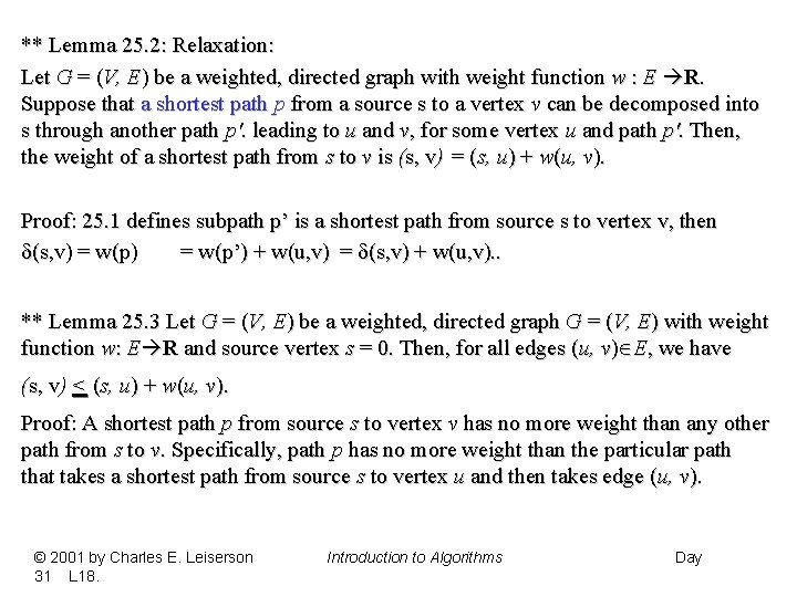
** Lemma 25. 2: Relaxation: Let G = (V, E) be a weighted, directed graph with weight function w : E R. Suppose that a shortest path p from a source s to a vertex v can be decomposed into s through another path p'. leading to u and v, for some vertex u and path p'. Then, the weight of a shortest path from s to v is (s, v) = (s, u) + w(u, v). Proof: 25. 1 defines subpath p’ is a shortest path from source s to vertex v, then (s, v) = w(p’) + w(u, v) = (s, v) + w(u, v). . ** Lemma 25. 3 Let G = (V, E) be a weighted, directed graph G = (V, E) with weight function w: E R and source vertex s = 0. Then, for all edges (u, v) E, we have (s, v) < (s, u) + w(u, v). Proof: A shortest path p from source s to vertex v has no more weight than any other path from s to v. Specifically, path p has no more weight than the particular path that takes a shortest path from source s to vertex u and then takes edge (u, v). © 2001 by Charles E. Leiserson 31 L 18. Introduction to Algorithms Day

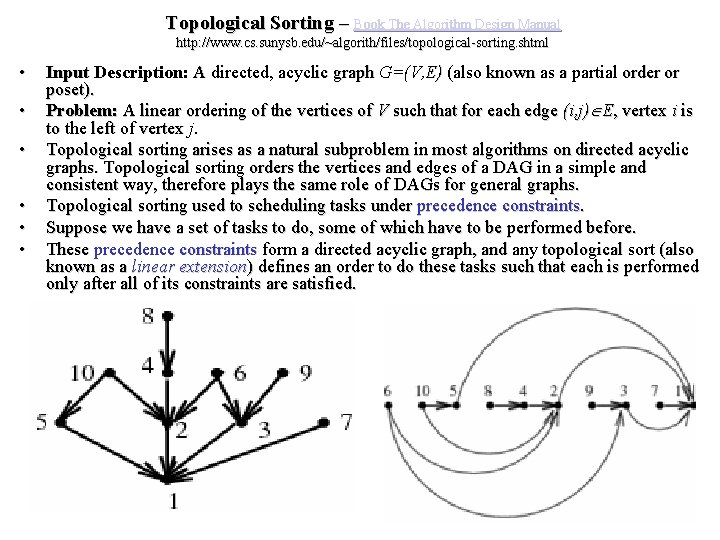
Topological Sorting – Book The Algorithm Design Manual http: //www. cs. sunysb. edu/~algorith/files/topological-sorting. shtml • • • Input Description: A directed, acyclic graph G=(V, E) (also known as a partial order or poset). Problem: A linear ordering of the vertices of V such that for each edge (i, j) E, vertex i is to the left of vertex j. Topological sorting arises as a natural subproblem in most algorithms on directed acyclic graphs. Topological sorting orders the vertices and edges of a DAG in a simple and consistent way, therefore plays the same role of DAGs for general graphs. Topological sorting used to scheduling tasks under precedence constraints. Suppose we have a set of tasks to do, some of which have to be performed before. These precedence constraints form a directed acyclic graph, and any topological sort (also known as a linear extension) defines an order to do these tasks such that each is performed only after all of its constraints are satisfied.

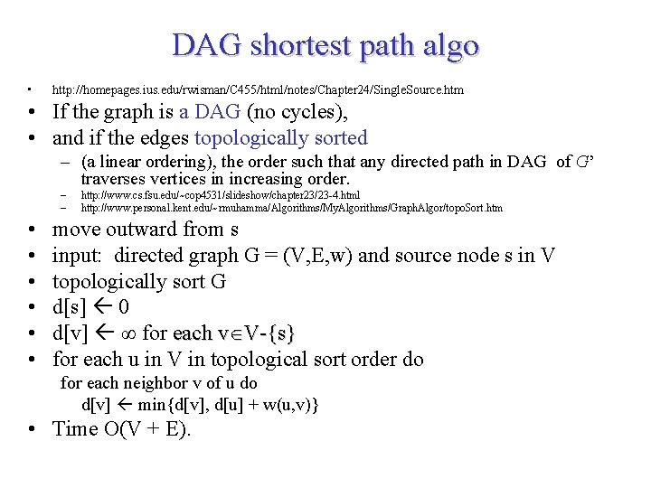
DAG shortest path algo • http: //homepages. ius. edu/rwisman/C 455/html/notes/Chapter 24/Single. Source. htm • If the graph is a DAG (no cycles), • and if the edges topologically sorted – (a linear ordering), the order such that any directed path in DAG of G’ traverses vertices in increasing order. – – • • • http: //www. cs. fsu. edu/~cop 4531/slideshow/chapter 23/23 -4. html http: //www. personal. kent. edu/~rmuhamma/Algorithms/My. Algorithms/Graph. Algor/topo. Sort. htm move outward from s input: directed graph G = (V, E, w) and source node s in V topologically sort G d[s] 0 d[v] ∞ for each v V-{s} for each u in V in topological sort order do for each neighbor v of u do d[v] min{d[v], d[u] + w(u, v)} • Time O(V + E).

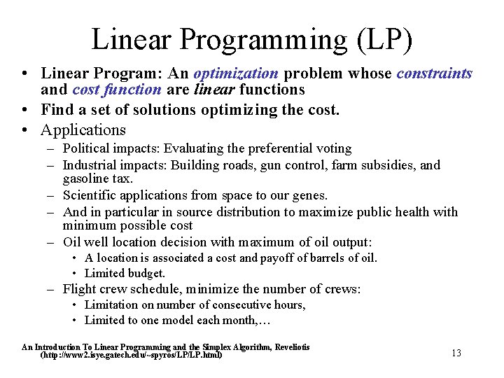
Linear Programming (LP) • Linear Program: An optimization problem whose constraints and cost function are linear functions • Find a set of solutions optimizing the cost. • Applications – Political impacts: Evaluating the preferential voting – Industrial impacts: Building roads, gun control, farm subsidies, and gasoline tax. – Scientific applications from space to our genes. – And in particular in source distribution to maximize public health with minimum possible cost – Oil well location decision with maximum of oil output: • A location is associated a cost and payoff of barrels of oil. • Limited budget. – Flight crew schedule, minimize the number of crews: • Limitation on number of consecutive hours, • Limited to one model each month, … An Introduction To Linear Programming and the Simplex Algorithm, Reveliotis (http: //www 2. isye. gatech. edu/~spyros/LP/LP. html) 13

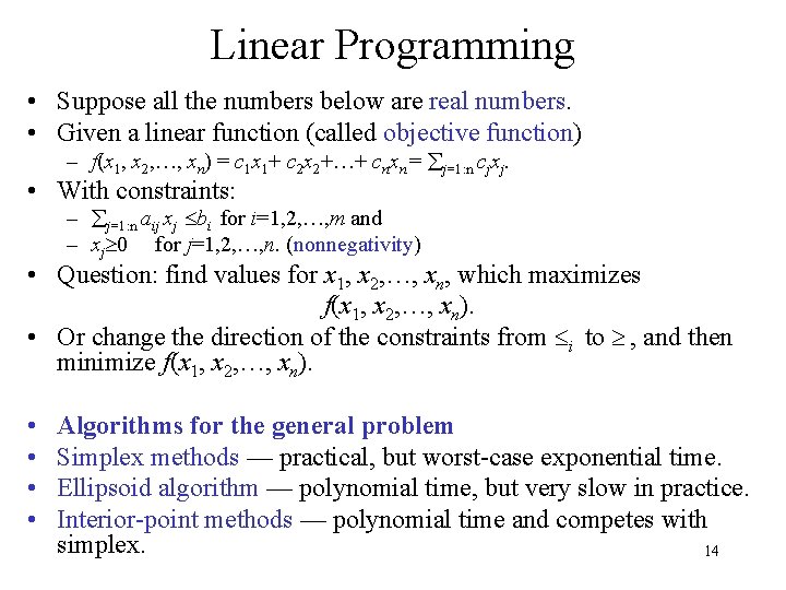
Linear Programming • Suppose all the numbers below are real numbers. • Given a linear function (called objective function) – f(x 1, x 2, …, xn) = c 1 x 1+ c 2 x 2+…+ cnxn = j=1: n cjxj. • With constraints: – j=1: n aij xj bi for i=1, 2, …, m and – xj 0 for j=1, 2, …, n. (nonnegativity) • Question: find values for x 1, x 2, …, xn, which maximizes f(x 1, x 2, …, xn). • Or change the direction of the constraints from i to , and then minimize f(x 1, x 2, …, xn). • • Algorithms for the general problem Simplex methods — practical, but worst-case exponential time. Ellipsoid algorithm — polynomial time, but very slow in practice. Interior-point methods — polynomial time and competes with simplex. 14

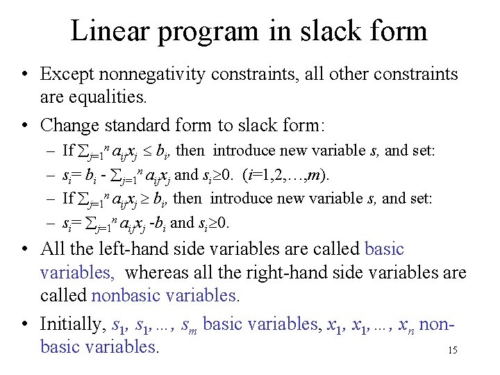
Linear program in slack form • Except nonnegativity constraints, all other constraints are equalities. • Change standard form to slack form: – – If j=1 n aijxj bi, then introduce new variable s, and set: si= bi - j=1 n aijxj and si 0. (i=1, 2, …, m). If j=1 n aijxj bi, then introduce new variable s, and set: si= j=1 n aijxj -bi and si 0. • All the left-hand side variables are called basic variables, whereas all the right-hand side variables are called nonbasic variables. • Initially, s 1, …, sm basic variables, x 1, …, xn nonbasic variables. 15

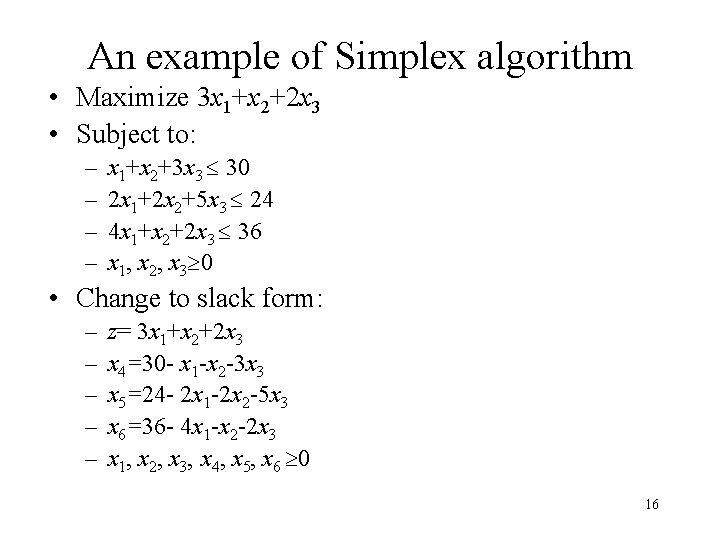
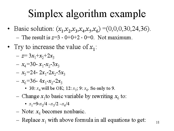
An example of Simplex algorithm • Maximize 3 x 1+x 2+2 x 3 • Subject to: – – x 1+x 2+3 x 3 30 2 x 1+2 x 2+5 x 3 24 4 x 1+x 2+2 x 3 36 x 1, x 2, x 3 0 • Change to slack form: – – – z= 3 x 1+x 2+2 x 3 x 4=30 - x 1 -x 2 -3 x 3 x 5=24 - 2 x 1 -2 x 2 -5 x 3 x 6=36 - 4 x 1 -x 2 -2 x 3 x 1, x 2, x 3, x 4, x 5, x 6 0 16

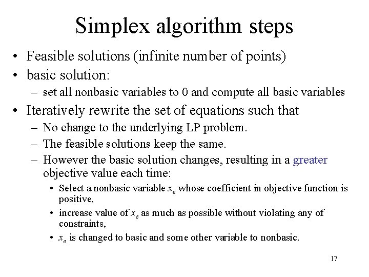
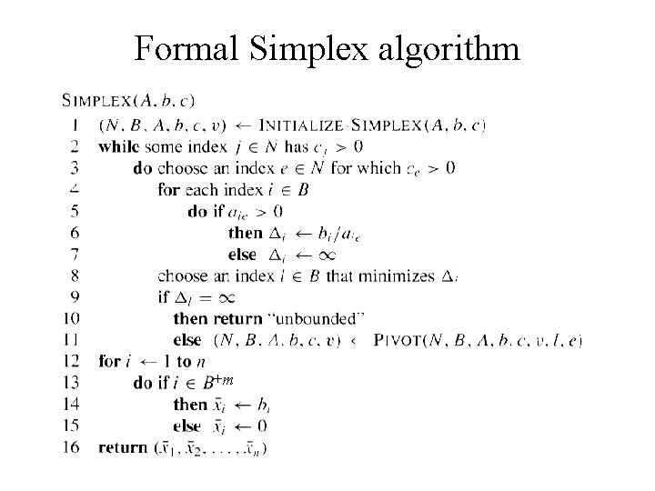
Simplex algorithm steps • Feasible solutions (infinite number of points) • basic solution: – set all nonbasic variables to 0 and compute all basic variables • Iteratively rewrite the set of equations such that – No change to the underlying LP problem. – The feasible solutions keep the same. – However the basic solution changes, resulting in a greater objective value each time: • Select a nonbasic variable xe whose coefficient in objective function is positive, • increase value of xe as much as possible without violating any of constraints, • xe is changed to basic and some other variable to nonbasic. 17

Simplex algorithm example • Basic solution: (x 1, x 2, x 3, x 4, x 5, x 6) =(0, 0, 0, 30, 24, 36). – The result is z=3 0+0+2 0=0. Not maximum. • Try to increase the value of x 1: – – z= 3 x 1+x 2+2 x 3 x 4=30 - x 1 -x 2 -3 x 3 x 5=24 - 2 x 1 -2 x 2 -5 x 3 x 6=36 - 4 x 1 -x 2 -2 x 3 • 30: x 4 will be OK; 12: x 5; 9: x 6. So only to 9. – Change x 1 to basic variable by rewriting x 6 to: • x 1=9 -x 2/4 –x 3/2 –x 6/4 – Note: x 6 becomes nonbasic. – Replace x 1 with above formula in all equations to get: 18

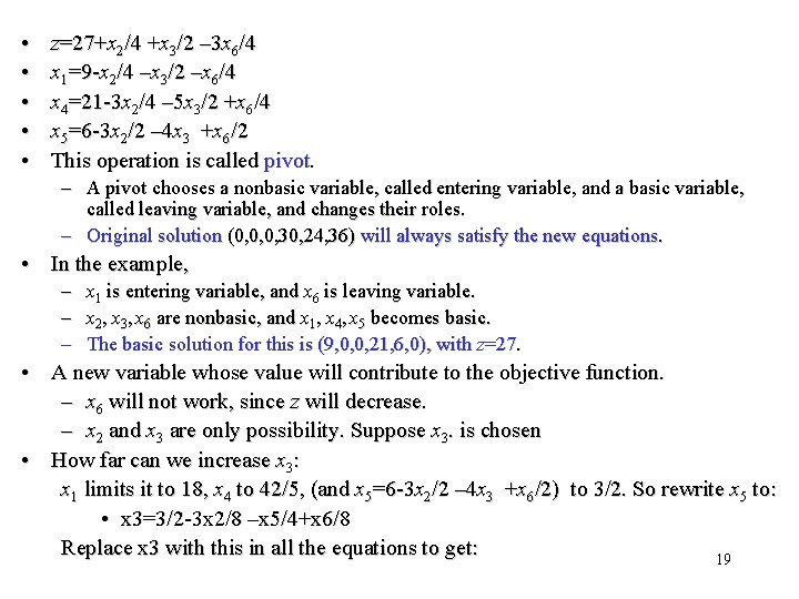
• • • z=27+x 2/4 +x 3/2 – 3 x 6/4 x 1=9 -x 2/4 –x 3/2 –x 6/4 x 4=21 -3 x 2/4 – 5 x 3/2 +x 6/4 x 5=6 -3 x 2/2 – 4 x 3 +x 6/2 This operation is called pivot. – A pivot chooses a nonbasic variable, called entering variable, and a basic variable, called leaving variable, and changes their roles. – Original solution (0, 0, 0, 30, 24, 36) will always satisfy the new equations. • In the example, – – – x 1 is entering variable, and x 6 is leaving variable. x 2, x 3, x 6 are nonbasic, and x 1, x 4, x 5 becomes basic. The basic solution for this is (9, 0, 0, 21, 6, 0), with z=27. • A new variable whose value will contribute to the objective function. – x 6 will not work, since z will decrease. – x 2 and x 3 are only possibility. Suppose x 3. is chosen • How far can we increase x 3: x 1 limits it to 18, x 4 to 42/5, (and x 5=6 -3 x 2/2 – 4 x 3 +x 6/2) to 3/2. So rewrite x 5 to: • x 3=3/2 -3 x 2/8 –x 5/4+x 6/8 Replace x 3 with this in all the equations to get: 19

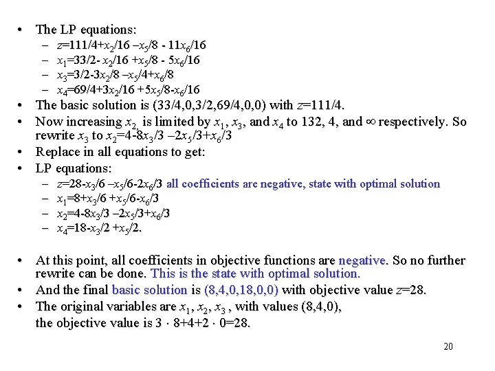
• The LP equations: – – • • z=111/4+x 2/16 –x 5/8 - 11 x 6/16 x 1=33/2 - x 2/16 +x 5/8 - 5 x 6/16 x 3=3/2 -3 x 2/8 –x 5/4+x 6/8 x 4=69/4+3 x 2/16 +5 x 5/8 -x 6/16 The basic solution is (33/4, 0, 3/2, 69/4, 0, 0) with z=111/4. Now increasing x 2, is limited by x 1, x 3, and x 4 to 132, 4, and respectively. So rewrite x 3 to x 2=4 -8 x 3/3 – 2 x 5/3+x 6/3 • Replace in all equations to get: • LP equations: – – z=28 -x 3/6 –x 5/6 -2 x 6/3 all coefficients are negative, state with optimal solution x 1=8+x 3/6 +x 5/6 -x 6/3 x 2=4 -8 x 3/3 – 2 x 5/3+x 6/3 x 4=18 -x 3/2 +x 5/2. • At this point, all coefficients in objective functions are negative. So no further rewrite can be done. This is the state with optimal solution. • And the final basic solution is (8, 4, 0, 18, 0, 0) with objective value z=28. • The original variables are x 1, x 2, x 3 , with values (8, 4, 0), the objective value is 3 8+4+2 0=28. 20

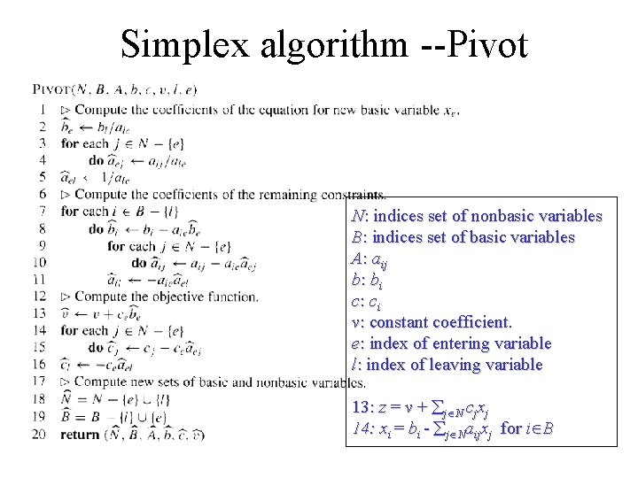
Simplex algorithm --Pivot N: indices set of nonbasic variables B: indices set of basic variables A: aij b: bi c: ci v: constant coefficient. e: index of entering variable l: index of leaving variable 13: z = v + j N cjxj 14: xi = bi - j Naijxj for i B

Formal Simplex algorithm +m 22

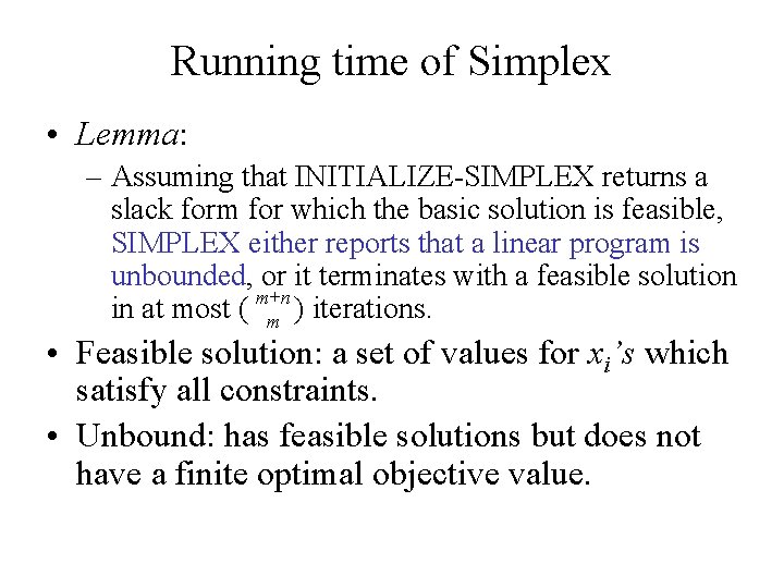
Running time of Simplex • Lemma: – Assuming that INITIALIZE-SIMPLEX returns a slack form for which the basic solution is feasible, SIMPLEX either reports that a linear program is unbounded, or it terminates with a feasible solution m+n in at most ( ) iterations. m • Feasible solution: a set of values for xi’s which satisfy all constraints. • Unbound: has feasible solutions but does not have a finite optimal objective value.

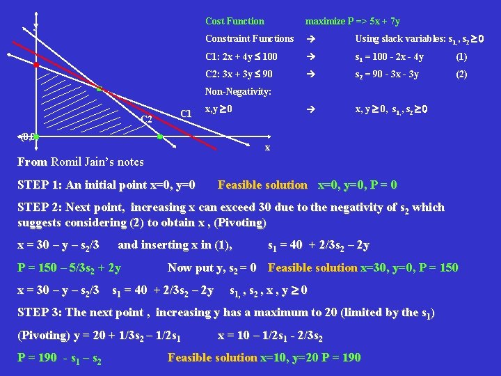
y Cost Function maximize P => 5 x + 7 y Constraint Functions Using slack variables: s 1, , s 2 ³ 0 C 1: 2 x + 4 y 100 s 1 = 100 - 2 x - 4 y (1) C 2: 3 x + 3 y 90 s 2 = 90 - 3 x - 3 y (2) x, y ³ 0, s 1, , s 2 ³ 0 Non-Negativity: C 2 C 1 x, y ³ 0 (0, 0) x From Romil Jain’s notes STEP 1: An initial point x=0, y=0 Feasible solution x=0, y=0, P = 0 STEP 2: Next point, increasing x can exceed 30 due to the negativity of s 2 which suggests considering (2) to obtain x , (Pivoting) x = 30 – y – s 2/3 and inserting x in (1), P = 150 – 5/3 s 2 + 2 y s 1 = 40 + 2/3 s 2 – 2 y Now put y, s 2 = 0 Feasible solution x=30, y=0, P = 150 x = 30 – y – s 2/3 s 1 = 40 + 2/3 s 2 – 2 y s 1, , s 2 , x , y ³ 0 STEP 3: The next point , increasing y has a maximum to 20 (limited by the s 1) (Pivoting) y = 20 + 1/3 s 2 – 1/2 s 1 P = 190 - s 1 – s 2 x = 10 – 1/2 s 1 - 2/3 s 2 Feasible solution x=10, y=20 P = 190

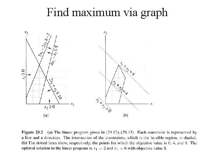
Find maximum via graph 25

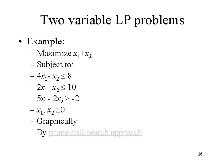
Two variable LP problems • Example: – Maximize x 1+x 2 – Subject to: – 4 x 1 - x 2 8 – 2 x 1+x 2 10 – 5 x 1 - 2 x 2 -2 – x 1, x 2 0 – Graphically – By prune-and-search approach 26

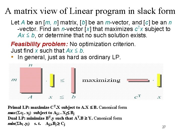
A matrix view of Linear program in slack form Let A be an [m, n] matrix, [b] be an m-vector, and [c] be an n -vector. Find an n-vector [x] that maximizes c. Tx subject to Ax ≤ b, or determine that no such solution exists. Feasibility problem: No optimization criterion. Just find x such that Ax ≤ b. • In general, just as hard as ordinary LP. Primal LP: maximize CT. X subject to A. X B. Canonical form max(Σcj. xj) subject to Aj, i. Xj Bj Dual LP: minimize BT. y such that AT. B ³ Y. Canonical form min(Σbi. yi) s. t. Aj, i. Bj ³ Cj 27

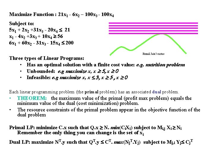
Maximize Function : 21 x 1 - 6 x 2 – 100 x 3 - 100 x 4 Subject to: 5 x 1 + 2 x 2 +31 x 3 - 20 x 4 21 x 1 - 4 x 2 +3 x 3 + 10 x 4 ³ 56 6 x 1 + 60 x 2 - 31 x 3 - 15 x 4 200 Romil Jain’s notes Three types of Linear Programs: • Has an optimal solution with a finite cost value: e. g. nutrition problem • Unbounded: e. g maximize x, x ³ 5, x ³ 0 • Infeasible: e. g maximize x, x 3, x ³ 5 , x ³ 0 Each linear programming problem (the primal problem) has an associated dual problem. • • THEOREM: the maximum value of the primal (profit max problem) equals the minimum value of the dual (cost minimization) problem. The resource constraints of the primal problem appear in the objective function of the dual problem Primal LP: minimize C. x such that Q. x ³ N. min(Ci. Xi) subject to Mi, j Xi ³ Ni Remember the only thing you can change is the set of xi Dual LP: maximize NT. y such that QT. y CT. max(Nj. T. Yj) subject to Mj, i Yj Cj. T

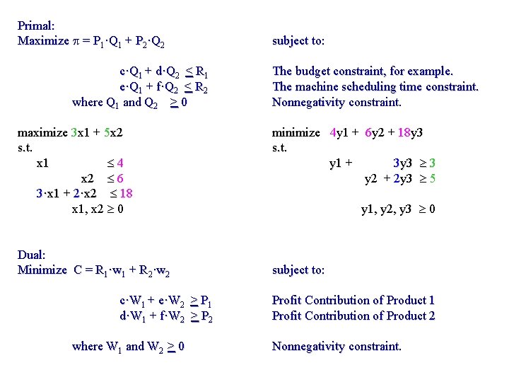
Primal: Maximize p = P 1·Q 1 + P 2·Q 2 subject to: c·Q 1 + d·Q 2 < R 1 e·Q 1 + f·Q 2 < R 2 where Q 1 and Q 2 > 0 The budget constraint, for example. The machine scheduling time constraint. Nonnegativity constraint. maximize 3 x 1 + 5 x 2 s. t. x 1 4 x 2 6 3·x 1 + 2·x 2 18 x 1, x 2 0 minimize 4 y 1 + 6 y 2 + 18 y 3 s. t. y 1 + 3 y 3 3 y 2 + 2 y 3 5 y 1, y 2, y 3 0 Dual: Minimize C = R 1·w 1 + R 2·w 2 subject to: c·W 1 + e·W 2 > P 1 d·W 1 + f·W 2 > P 2 where W 1 and W 2 > 0 Profit Contribution of Product 1 Profit Contribution of Product 2 Nonnegativity constraint.

• Each constraint has an implicit price, the shadow price of the constraint. If a constraint is slack, its shadow price is zero. • Each shadow price has much the same meaning as a Lagrangian multiplier. Cost Minimization Problem Using Linear Programming • Multi-plant firms want to produce with the lowest cost across their disparate facilities. Sometimes, the relative efficiencies of the different plants can be exploited to reduce costs. • A firm may have two mines that produces different qualities of ore. The firm has output requirements in each ore quality. • Scheduling of hours per week in each mine has the objective of minimizing cost, but achieving the required outputs. • If one mine is more efficient in all categories of ore, and is less costly to operate, the optimal solution may involve shutting one mine down. • The dual of this problem involves the shadow prices of the ore constraints. It tells the implicit value of each quality of ore. Capital Rationing Problem: Financial decisions sometimes may be viewed as a linear programming problem. • A financial officer may want to maximize the return on investments available, given a limited amount of money to invest. • The usual problem in finance is to accept all projects with positive net present values, but sometimes the capital budgets are fixed or limited to create "capital rationing" among projects. • The solution involves determining what fraction of money allotted should be invested in each of the possible projects or investments. • In some problems, projects cannot be broken into small parts. • When this is the case, integer programming can be added to the problem.

• A linear program problem with additional constraint that all variables must take integer!!! values. – Given an integer mxn matrix A and an integer m-vector b, whethere is an integer n-vector x such that Ax<=b. – this problem is NP-complete. • However the general linear program problem is poly time solvable. 31

Complexity of simplex and LP complete • Usually runs quickly in practice. However, note in the worst-case the simplex method takes exponential time. The Klee-Minty Cube is an example LP problem the simplex taking exponential running time. This is a perturbation of an n-dimensional cube having about 2 n vertices. For most pivot choices the simplex method will visit all of these vertices in 2 n-1 pivot steps to find the optimal solution. • Some linear programming algorithms that do have polynomial bounds in the worst-case will also be mentioned. • The LP-Complete class of problems is the set of problems X such that: – the problem can be formulated as an instance of a LP, this means that there is a polynomial-time deterministic algorithm that transforms instances of the problem X into instances of linear programs. So, first converting it into an LP problem in polynomial time and then solving LP problem. – the problem is LP-hard. This is analogous to the definition for NP-Complete problems. Means that there is a polynomial-time deterministic algorithm converting any instance of an LP problem into an instance of problem type X. The LP-complete class of problems is polynomial-time solvable, i. e. P = LP.

Simplex method traverses the boundary of the polyhedron along its edges, so its running time depends on the complexity of the polyhedron, even though we don’t really care about the polyhedron but are only interested in one of its vertices. The ellipsoid method always remains outside of the polyhedron, and keeps on shrinking the ellipsoid until it finds a point inside the polyhedron. So one could think of the ellipsoid method as an exterior point method. Instead, interior point methods always remaining inside the polyhedron, by starting inside and following a path to the boundary. This means the complexity of these methods does not really depend on the complexity of the polyhedron. Among many of the interior point methods, log barrier method. Simulating a force at the boundary repelling the path in order to keep solution sought inside the polyhedron at all times. But initially the force is very strong, which restricts the search to a small area in the center of the polyhedron, and the force weakens with time to allow the path to eventually reach the boundary and find the optimal vertex of the polyhedron.

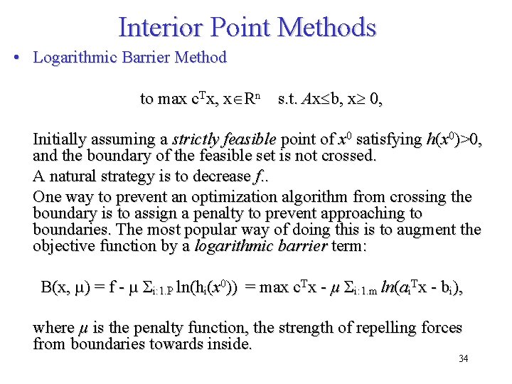
Interior Point Methods • Logarithmic Barrier Method to max c. Tx, x Rn s. t. Ax b, x 0, Initially assuming a strictly feasible point of x 0 satisfying h(x 0)>0, and the boundary of the feasible set is not crossed. A natural strategy is to decrease f. . One way to prevent an optimization algorithm from crossing the boundary is to assign a penalty to prevent approaching to boundaries. The most popular way of doing this is to augment the objective function by a logarithmic barrier term: B(x, µ) = f - µ Σi: 1. P ln(hi(x 0)) = max c. Tx - µ Σi: 1. m ln(ai. Tx - bi), where µ is the penalty function, the strength of repelling forces from boundaries towards inside. 34

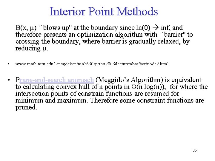
Interior Point Methods B(x, µ) ``blows up'' at the boundary since ln(0) inf, and therefore presents an optimization algorithm with ``barrier'' to crossing the boundary, where barrier is gradually relaxed, by reducing µ. • www. math. mtu. edu/~msgocken/ma 5630 spring 2003/lectures/bar/node 2. html • Prune-and-search approach (Meggido’s Algorithm) is equivalent to calculating convex hull of n points in O(n log(n)), for where the intersection points of constrain functions are resumed for minimum and maximum. Therefore some constraint functions are pruned. 35

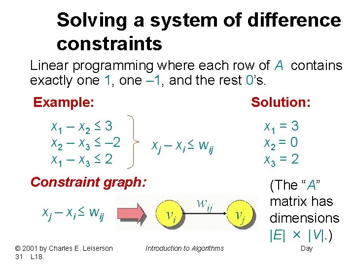
Solving a system of difference constraints Linear programming where each row of A contains exactly one 1, one – 1, and the rest 0’s. Example: Solution: x 1 – x 2 ≤ 3 x 2 – x 3 ≤ – 2 x 1 – x 3 ≤ 2 xj – xi ≤ wij Constraint graph: xj – xi ≤ wij © 2001 by Charles E. Leiserson 31 L 18. Introduction to Algorithms x 1 = 3 x 2 = 0 x 3 = 2 (The “A” matrix has dimensions |E| × |V|. ) Day

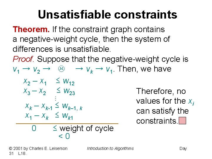
Unsatisfiable constraints Theorem. If the constraint graph contains a negative-weight cycle, then the system of differences is unsatisfiable. Proof. Suppose that the negative-weight cycle is v 1 → v 2 → → vk → v 1. Then, we have x 2 – x 1 ≤ w 12 x 3 – x 2 ≤ w 23 Therefore, no values for the xi xk – xk-1 ≤ wk– 1, k can satisfy the x 1 – xk ≤ wk 1 constraints. 0 ≤ weight of cycle <0 © 2001 by Charles E. Leiserson 31 L 18. Introduction to Algorithms Day

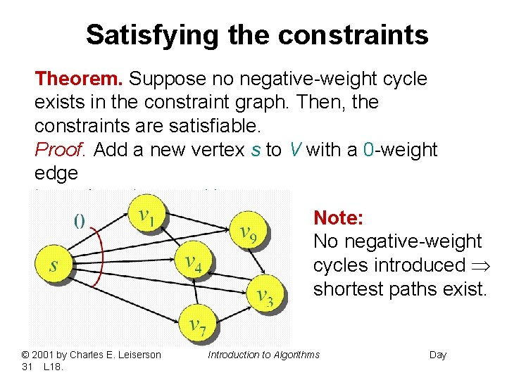
Satisfying the constraints Theorem. Suppose no negative-weight cycle exists in the constraint graph. Then, the constraints are satisfiable. Proof. Add a new vertex s to V with a 0 -weight edge to each vertex vi V. Note: No negative-weight cycles introduced shortest paths exist. © 2001 by Charles E. Leiserson 31 L 18. Introduction to Algorithms Day

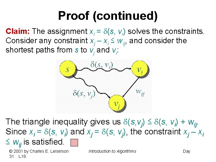
Proof (continued) Claim: The assignment xi = (s, vi) solves the constraints. Consider any constraint xj – xi ≤ wij, and consider the shortest paths from s to vj and vi: The triangle inequality gives us (s, vj) ≤ (s, vi) + wij. Since xi = (s, vi) and xj = (s, vj), the constraint xj – xi ≤ wij is satisfied. © 2001 by Charles E. Leiserson 31 L 18. Introduction to Algorithms Day

Bellman-Ford and linear programming Corollary. The Bellman-Ford algorithm can solve a system of m difference constraints on n variables in O(mn) time. Single-source shortest paths is a simple LP problem. … In fact, Bellman-Ford maximizes x 1 + x 2 + + xn subject to the constraints xj – xi ≤ wij and xi ≤ 0. Bellman-Ford also minimizes maxi{xi} – mini{xi}. © 2001 by Charles E. Leiserson 31 L 18. Introduction to Algorithms Day

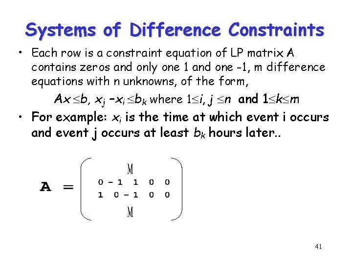
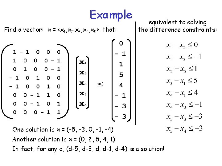
Systems of Difference Constraints • Each row is a constraint equation of LP matrix A contains zeros and only one 1 and one -1, m difference equations with n unknowns, of the form, Ax b, xj –xi bk where 1 i, j n and 1 k m • For example: xi is the time at which event i occurs and event j occurs at least bk hours later. . 41

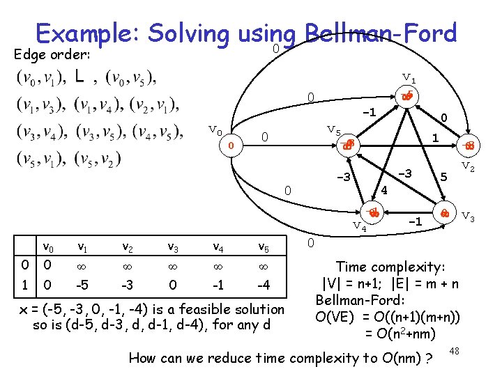
Example Find a vector: x = <x 1, x 2 x 3, x 4, x 5> that: equivalent to solving the difference constraints: One solution is x = (-5, -3, 0, -1, -4) Another solution is x = (0, 2, 5, 4, 1) In fact, for any d, (d-5, d-3, d, d-1, d-4) is a solution!

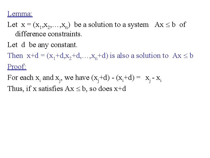
Lemma: Let x = (x 1, x 2, …, xn) be a solution to a system Ax b of difference constraints. Let d be any constant. Then x+d = (x 1+d, x 2+d, …, xn+d) is also a solution to Ax b Proof: For each xi and xj, we have (xj+d) - (xi+d) = xj - xi Thus, if x satisfies Ax b, so does x+d

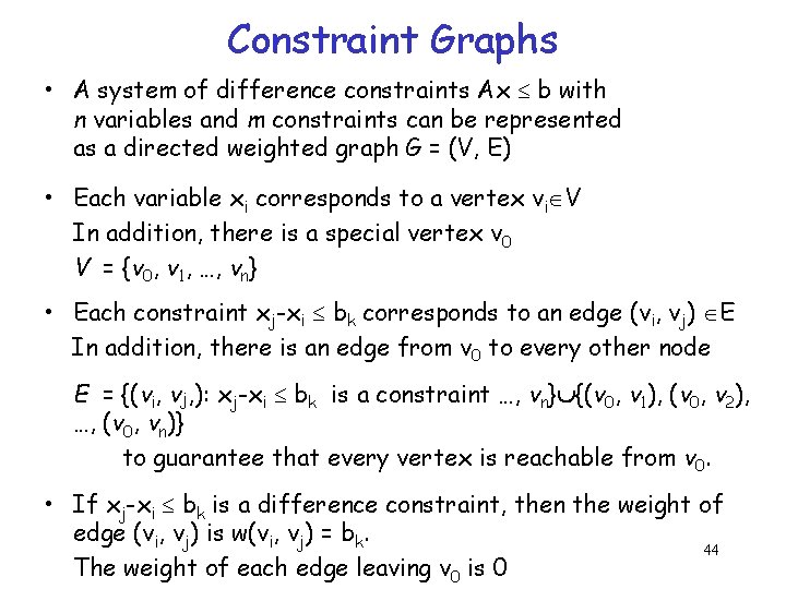
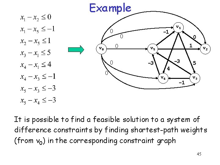
Constraint Graphs • A system of difference constraints Ax b with n variables and m constraints can be represented as a directed weighted graph G = (V, E) • Each variable xi corresponds to a vertex vi V In addition, there is a special vertex v 0 V = {v 0, v 1, …, vn} • Each constraint xj-xi bk corresponds to an edge (vi, vj) E In addition, there is an edge from v 0 to every other node E = {(vi, vj, ): xj-xi bk is a constraint …, vn} {(v 0, v 1), (v 0, v 2), …, (v 0, vn)} to guarantee that every vertex is reachable from v 0. • If xj-xi bk is a difference constraint, then the weight of edge (vi, vj) is w(vi, vj) = bk. 44 The weight of each edge leaving v 0 is 0

Example 0 0 0 v 0 0 0 -1 v 1 0 1 v 5 -3 -3 4 v 4 -1 v 2 5 v 3 It is possible to find a feasible solution to a system of difference constraints by finding shortest-path weights (from v 0) in the corresponding constraint graph 45

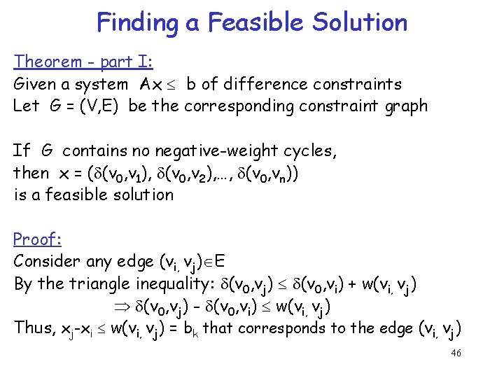
Finding a Feasible Solution Theorem - part I: Given a system Ax b of difference constraints Let G = (V, E) be the corresponding constraint graph If G contains no negative-weight cycles, then x = ( (v 0, v 1), (v 0, v 2), …, (v 0, vn)) is a feasible solution Proof: Consider any edge (vi, vj) E By the triangle inequality: (v 0, vj) (v 0, vi) + w(vi, vj) (v 0, vj) - (v 0, vi) w(vi, vj) Thus, xj-xi w(vi, vj) = bk that corresponds to the edge (vi, vj) 46

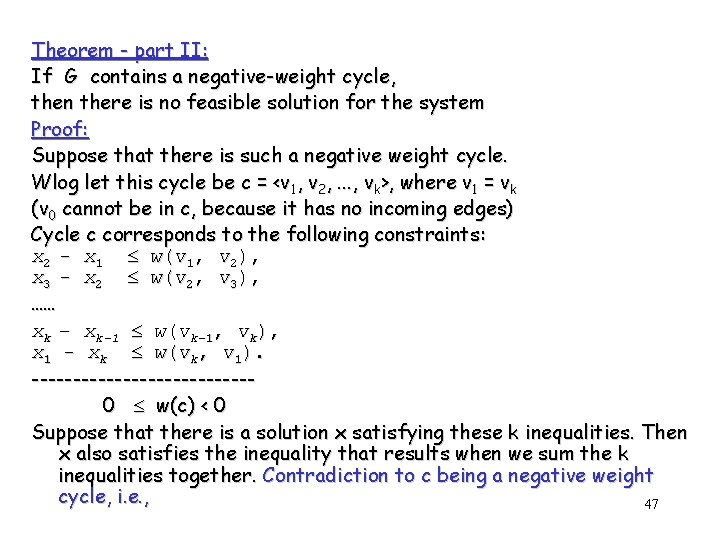
Theorem - part II: If G contains a negative-weight cycle, then there is no feasible solution for the system Proof: Suppose that there is such a negative weight cycle. Wlog let this cycle be c = <v 1, v 2, . . . , vk>, where v 1 = vk (v 0 cannot be in c, because it has no incoming edges) Cycle c corresponds to the following constraints: x 2 - x 1 w(v 1, v 2), x 3 - x 2 w(v 2, v 3), …… xk – xk-1 w(vk-1, vk), x 1 - xk w(vk, v 1). -------------0 w(c) < 0 Suppose that there is a solution x satisfying these k inequalities. Then x also satisfies the inequality that results when we sum the k inequalities together. Contradiction to c being a negative weight cycle, i. e. , 47

Example: Solving using Bellman-Ford 0 Edge order: v 1 -5 0 0 v 0 0 -1 v 5 0 1 -4 -3 0 -3 -3 0 4 -1 0 v 4 v 0 v 1 v 2 v 3 v 4 v 5 0 0 ∞ ∞ ∞ 1 0 -5 -3 0 -1 -4 0 x = (-5, -3, 0, -1, -4) is a feasible solution so is (d-5, d-3, d, d-1, d-4), for any d -1 -3 0 v 2 5 0 v 3 0 Time complexity: |V| = n+1; |E| = m + n Bellman-Ford: O(VE) = O((n+1)(m+n)) = O(n 2+nm) How can we reduce time complexity to O(nm) ? 48

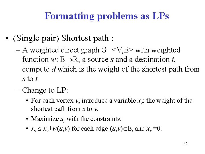
Formatting problems as LPs • (Single pair) Shortest path : – A weighted direct graph G=<V, E> with weighted function w: E R, a source s and a destination t, compute d which is the weight of the shortest path from s to t. – Change to LP: • For each vertex v, introduce a variable xv: the weight of the shortest path from s to v. • Maximize xt with the constraints: • xv xu+w(u, v) for each edge (u, v) E, and xs =0. 49

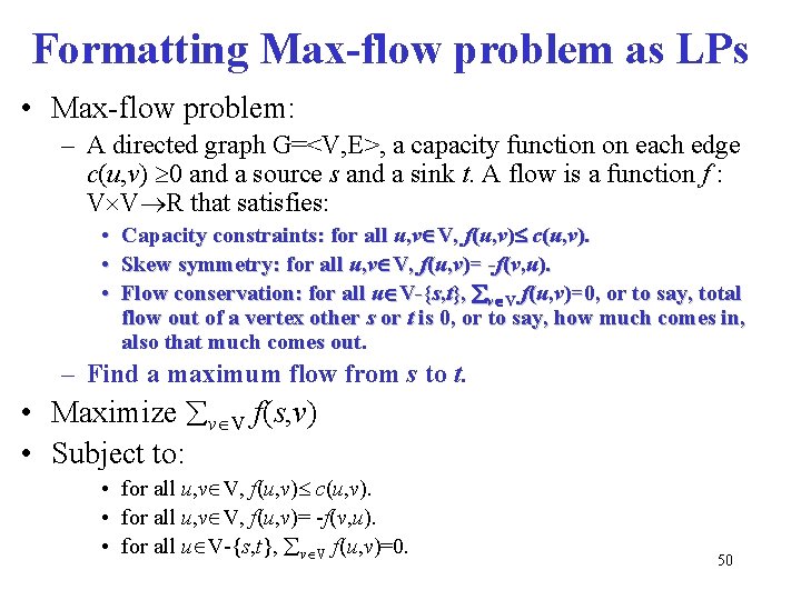
Formatting Max-flow problem as LPs • Max-flow problem: – A directed graph G=<V, E>, a capacity function on each edge c(u, v) 0 and a source s and a sink t. A flow is a function f : V V R that satisfies: • • • Capacity constraints: for all u, v V, f(u, v) c(u, v). Skew symmetry: for all u, v V, f(u, v)= -f(v, u). Flow conservation: for all u V-{s, t}, v V f(u, v)=0, or to say, total flow out of a vertex other s or t is 0, or to say, how much comes in, also that much comes out. – Find a maximum flow from s to t. • Maximize v V f(s, v) • Subject to: • for all u, v V, f(u, v) c(u, v). • for all u, v V, f(u, v)= -f(v, u). • for all u V-{s, t}, v V f(u, v)=0. 50

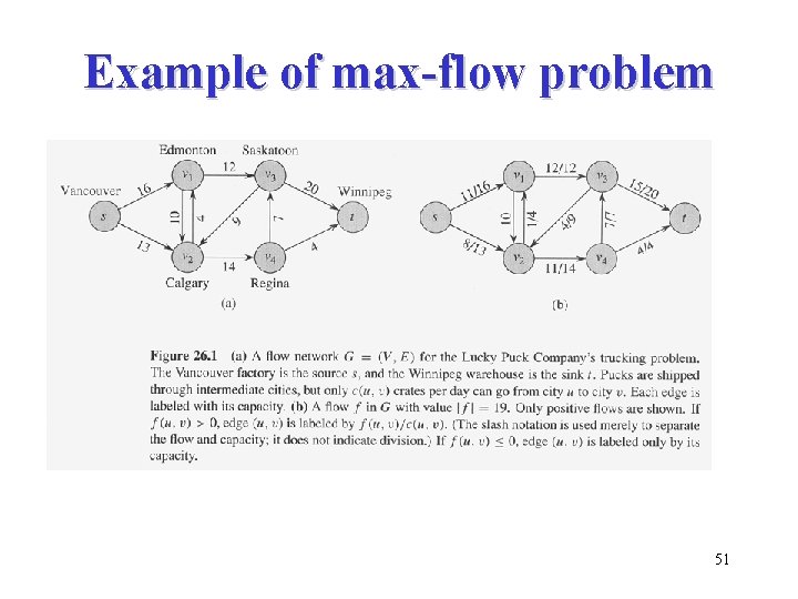
Example of max-flow problem 51

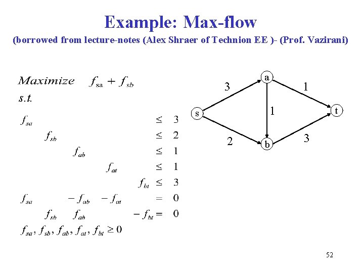
Example: Max-flow (borrowed from lecture-notes (Alex Shraer of Technion EE )- (Prof. Vazirani) 3 s. t. a 1 1 s 2 b t 3 52

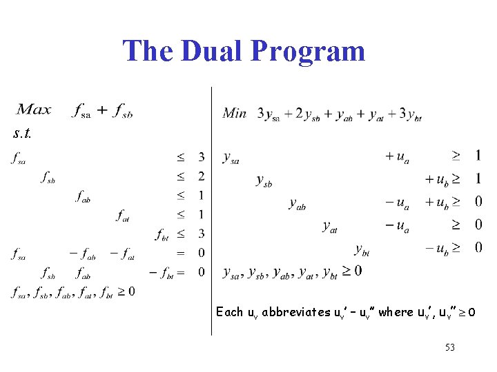
The Dual Program s. t. Each uv abbreviates uv’ – uv’’ where uv’, uv’’ 0 53

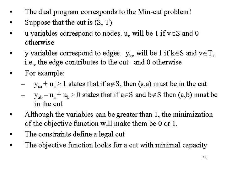
• • The dual program corresponds to the Min-cut problem! Suppose that the cut is (S, T) u variables correspond to nodes. uv will be 1 if v S and 0 otherwise y variables correspond to edges. ykv will be 1 if k S and v T, i. e. , the edge contributes to the cut and 0 otherwise For example: – ysa + ua 1 states that if a S, then (s, a) must be in the cut – yab – ua + ub 0 states that if a S and b S then (a, b) must be in the cut Although the variables can be greater than 1, the minimization of the objective function will make them be 0 or 1. The constraints define a legal cut The objective function looks for a cut with minimal capacity 54

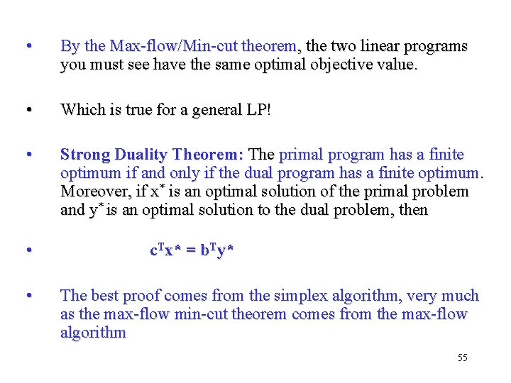
• By the Max-flow/Min-cut theorem, the two linear programs you must see have the same optimal objective value. • Which is true for a general LP! • Strong Duality Theorem: The primal program has a finite optimum if and only if the dual program has a finite optimum. Moreover, if x* is an optimal solution of the primal problem and y* is an optimal solution to the dual problem, then • • c. Tx* = b. Ty* The best proof comes from the simplex algorithm, very much as the max-flow min-cut theorem comes from the max-flow algorithm 55