Single Period Inventory Models Yossi Sheffi Mass Inst

Single Period Inventory Models Yossi Sheffi Mass Inst of Tech Cambridge, MA

Outline • Single period inventory decisions • Calculating the optimal order size • � Numerically • Using spreadsheet • Using simulation • • • � Analytically The profit function � For specific distribution Level of Service Extensions: � Fixed costs � Risks � Initial inventory � Elastic demand

Single Period Ordering • • • Seasonal items Perishable goods News print Fashion items Some high tech products Risky investments

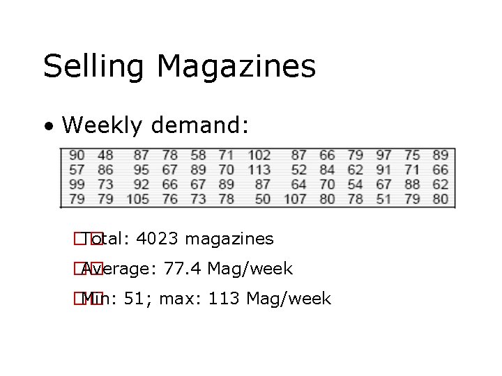
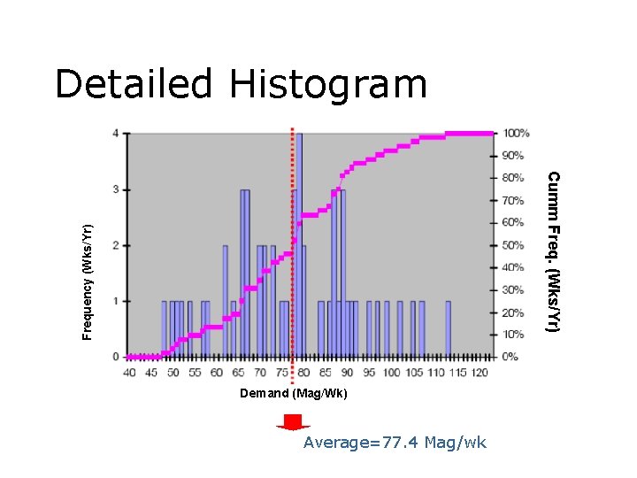
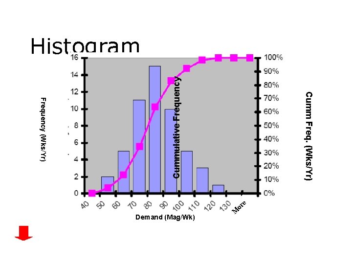
Selling Magazines • Weekly demand: �� Total: 4023 magazines �� Average: 77. 4 Mag/week �� Min: 51; max: 113 Mag/week

Detailed Histogram Frequency (Wks/Yr) Cumm Freq. (Wks/Yr) Demand (Mag/Wk) Average=77. 4 Mag/wk

M Demand (Mag/Wk) or e Cumm Freq. (Wks/Yr) Frequency (Wks/Yr) Cummulative Frequency Histogram

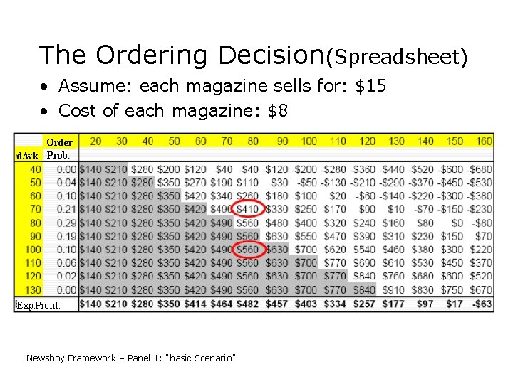
The Ordering Decision(Spreadsheet) • Assume: each magazine sells for: $15 • Cost of each magazine: $8 Order d/wk Prob Exp. Profit: Newsboy Framework – Panel 1: “basic Scenario”

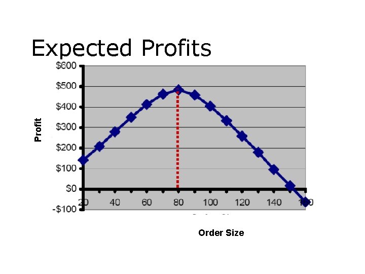
Profit Expected Profits Order Size

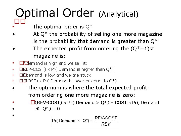
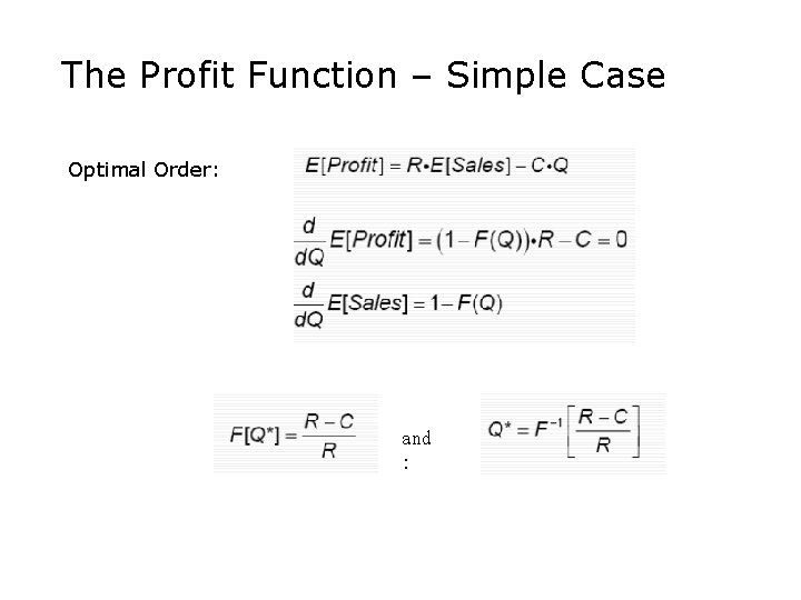
Optimal Order �� • • • (Analytical) The optimal order is Q* At Q* the probability of selling one more magazine is the probability that demand is greater than Q* The expected profit from ordering the (Q*+1)st magazine is: • �� If demand is high and we sell it: • • �� (REV-COST) x Pr( Demand is higher than Q*) �� If demand is low and we are stuck: �� (-COST) x Pr( Demand is lower or equal to Q*) The optimum is where the total expected profit from ordering one more magazine is zero: �(REV-COST) x Pr( Demand > Q*) – COST x Pr( Demand ≤ Q*) = 0

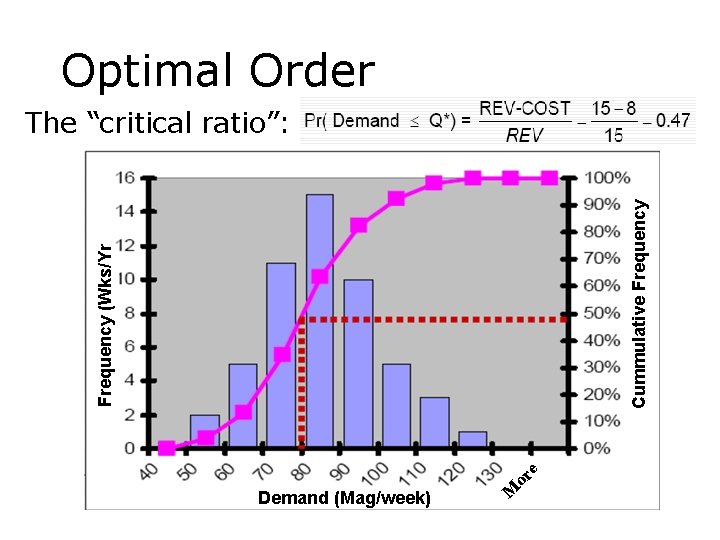
Optimal Order M Demand (Mag/week) or e Frequency (Wks/Yr Cummulative Frequency The “critical ratio”:

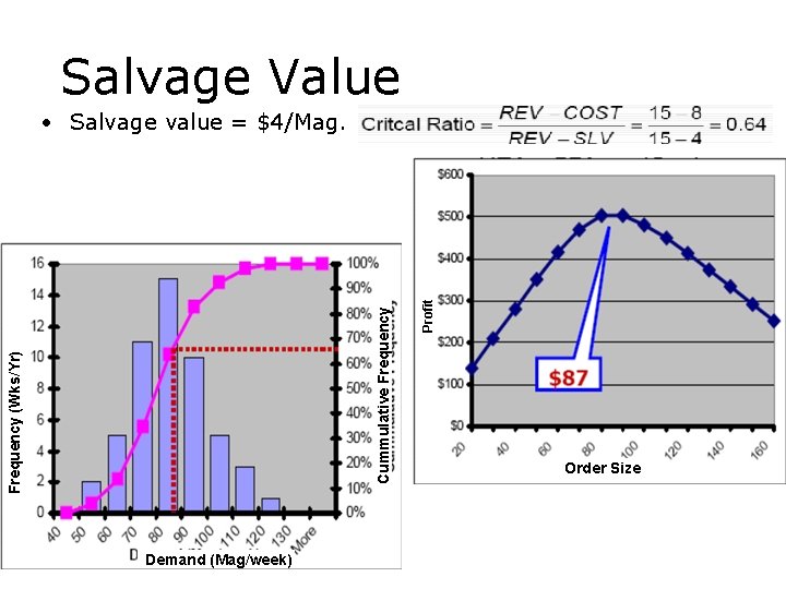
Salvage Value Frequency (Wks/Yr) Demand (Mag/week) Profit Cummulative Frequency • Salvage value = $4/Mag. Order Size

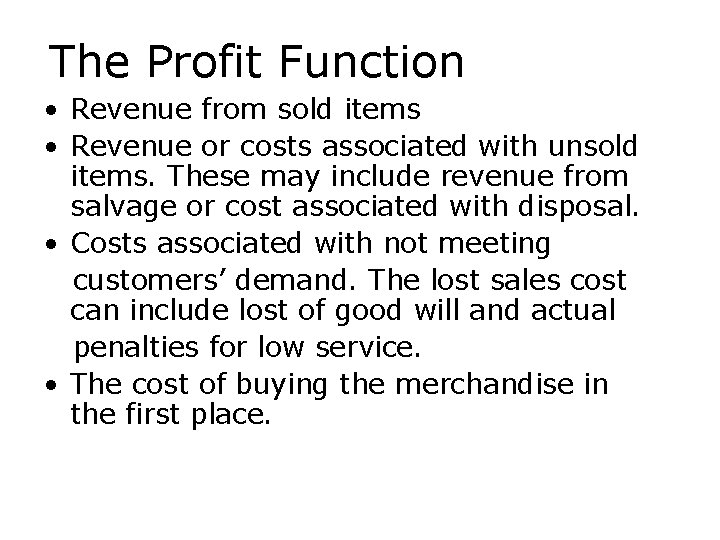
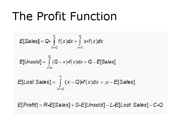
The Profit Function • Revenue from sold items • Revenue or costs associated with unsold items. These may include revenue from salvage or cost associated with disposal. • Costs associated with not meeting customers’ demand. The lost sales cost can include lost of good will and actual penalties for low service. • The cost of buying the merchandise in the first place.

The Profit Function

The Profit Function – Simple Case Optimal Order: and :

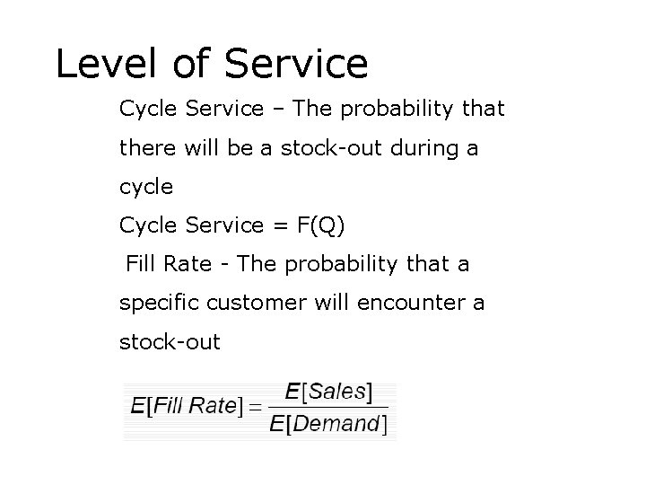
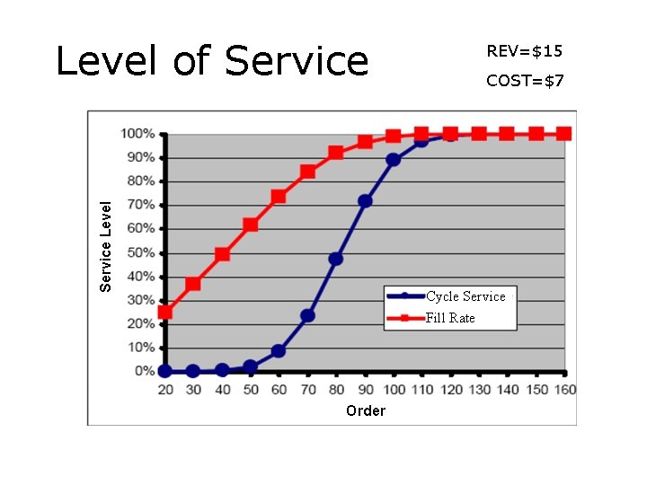
Level of Service Cycle Service – The probability that there will be a stock-out during a cycle Cycle Service = F(Q) Fill Rate - The probability that a specific customer will encounter a stock-out

Service Level of Service REV=$15 COST=$7 Cycle Service Fill Rate Order

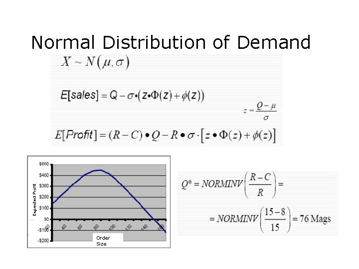
Expected Profit Normal Distribution of Demand Order Size

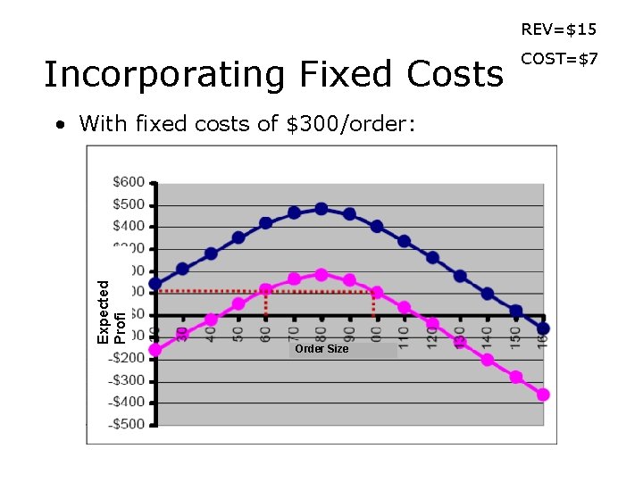
REV=$15 Incorporating Fixed Costs Expected Profi • With fixed costs of $300/order: Order Size COST=$7

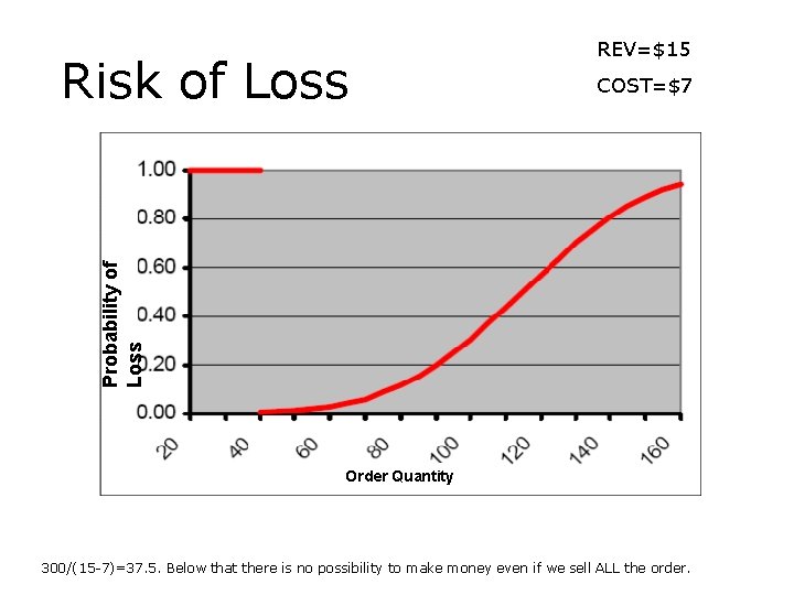
COST=$7 Probability of Loss Risk of Loss REV=$15 Order Quantity 300/(15 -7)=37. 5. Below that there is no possibility to make money even if we sell ALL the order.

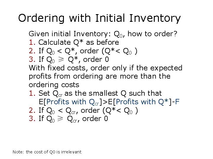
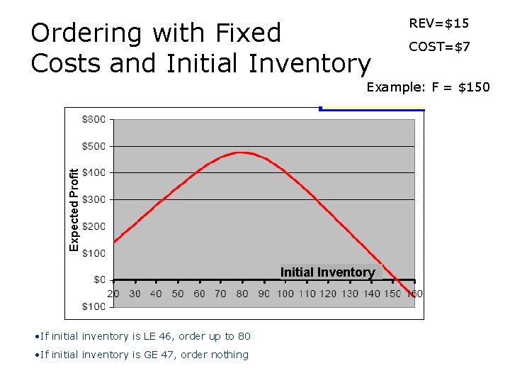
Ordering with Initial Inventory Given initial Inventory: Q 0, how to order? 1. Calculate Q* as before 2. If Q 0 < Q*, order (Q*< Q 0 ) 3. If Q 0 ≥ Q*, order 0 With fixed costs, order only if the expected profits from ordering are more than the ordering costs 1. Set Qcr as the smallest Q such that E[Profits with Qcr]>E[Profits with Q*]-F 2. If Q 0 < Qcr, order (Q*< Q 0 ) 3. If Q 0 ≥ Qcr, order 0 Note: the cost of Q 0 is irrelevant

Ordering with Fixed Costs and Initial Inventory REV=$15 COST=$7 Expected Profit Example: F = $150 Initial Inventory • If initial inventory is LE 46, order up to 80 • If initial inventory is GE 47, order nothing

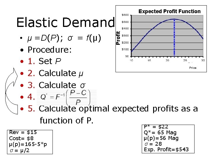
• • Profit Elastic Demand Expected Profit Function μ =D(P); σ = f(μ) Procedure: 1. Set P 2. Calculate μ 3. Calculate σ 4. 5. Calculate optimal expected profits as a function of P. Rev = $15 Cost= $8 μ(p)=165 -5*p σ= μ/2 Price P* = $22 Q*= 65 Mag μ(p)=56 Mag σ= 28 Exp. Profit=$543

Any Questions? Yossi Sheffi