Single Cell Sequencing Analysis Single Cell Sequencing Data

Single Cell Sequencing Analysis

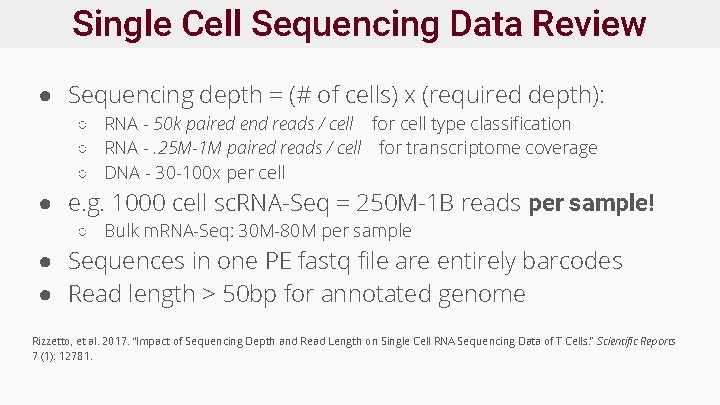
Single Cell Sequencing Data Review ● Sequencing depth = (# of cells) x (required depth): ○ RNA - 50 k paired end reads / cell for cell type classification ○ RNA -. 25 M-1 M paired reads / cell for transcriptome coverage ○ DNA - 30 -100 x per cell ● e. g. 1000 cell sc. RNA-Seq = 250 M-1 B reads per sample! ○ Bulk m. RNA-Seq: 30 M-80 M per sample ● Sequences in one PE fastq file are entirely barcodes ● Read length > 50 bp for annotated genome Rizzetto, et al. 2017. “Impact of Sequencing Depth and Read Length on Single Cell RNA Sequencing Data of T Cells. ” Scientific Reports 7 (1): 12781.

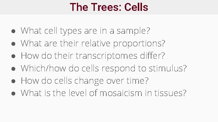
The Trees: Cells ● ● ● What cell types are in a sample? What are their relative proportions? How do their transcriptomes differ? Which/how do cells respond to stimulus? How do cells change over time? What is the level of mosaicism in tissues?

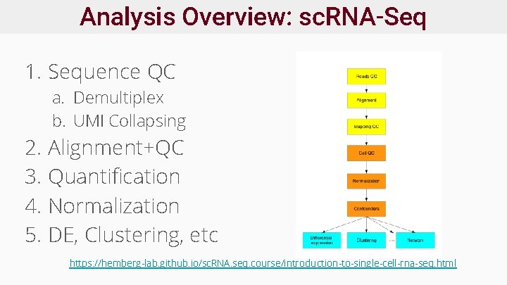
Analysis Overview: sc. RNA-Seq 1. Sequence QC a. Demultiplex b. UMI Collapsing 2. Alignment+QC 3. Quantification 4. Normalization 5. DE, Clustering, etc https: //hemberg-lab. github. io/sc. RNA. seq. course/introduction-to-single-cell-rna-seq. html

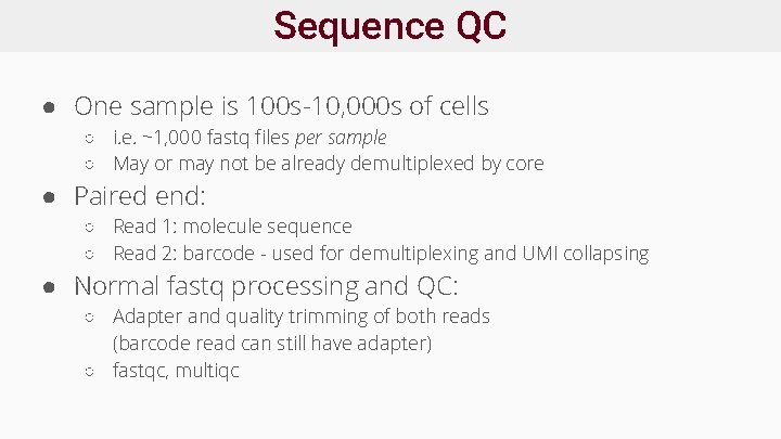
Sequence QC ● One sample is 100 s-10, 000 s of cells ○ i. e. ~1, 000 fastq files per sample ○ May or may not be already demultiplexed by core ● Paired end: ○ Read 1: molecule sequence ○ Read 2: barcode - used for demultiplexing and UMI collapsing ● Normal fastq processing and QC: ○ Adapter and quality trimming of both reads (barcode read can still have adapter) ○ fastqc, multiqc

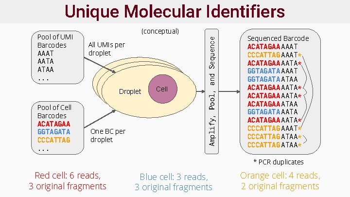
Unique Molecular Identifiers ● Enable detection of q. PCR amp. artefacts ● Not required, but often used ● Reads deduplicated or collapsed by cell barcode+UMI sequence prior to analysis ● Barcodes/UMIs designed to tolerate sequencing errors ○ i. e. >2 edit distance between any two sequences

Unique Molecular Identifiers (conceptual) All UMIs per droplet Droplet Pool of Cell Barcodes ACATAGAA GGTAGATA CCCATTAG. . . One BC per droplet Droplet Cell Amplify, Pool, and Sequence Pool of UMI Barcodes AAAT AATA ATAA. . . Sequenced Barcode ACATAGAA AAAT CCCATTAG AAAT* ACATAGAA AATA* GGTAGATA AAAT GGTAGATA ATAA ACATAGAA AATA* ACATAGAA ATAA GGTAGATA ACATAGAA AATA* CCCATTAG AAAT* CCCATTAG ATAA* * PCR duplicates Red cell: 6 reads, 3 original fragments Blue cell: 3 reads, 3 original fragments Orange cell: 4 reads, 2 original fragments

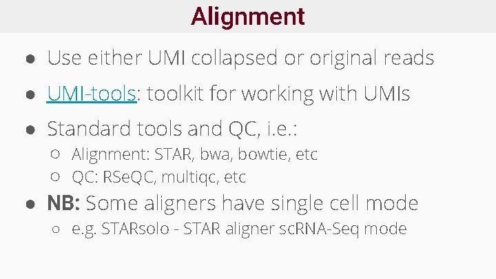
Alignment ● Use either UMI collapsed or original reads ● UMI-tools: toolkit for working with UMIs ● Standard tools and QC, i. e. : ○ Alignment: STAR, bwa, bowtie, etc ○ QC: RSe. QC, multiqc, etc ● NB: Some aligners have single cell mode ○ e. g. STARsolo - STAR aligner sc. RNA-Seq mode

QC: Mitochondria and spike-in controls ● High % reads mapping to mitochondrial genes = indicates low sample quality ● Spike-in (synthetic) RNA is sometimes used as an alternative control ● Idea: if mito/spike-in reads make up high proportion of reads, m. RNA concentration was low

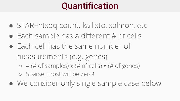
Quantification ● STAR+htseq-count, kallisto, salmon, etc ● Each sample has a different # of cells ● Each cell has the same number of measurements (e. g. genes) ○ = (# of samples) x (# of cells) x (# of genes) ○ Sparse: most will be zero! ● We consider only single sample case below

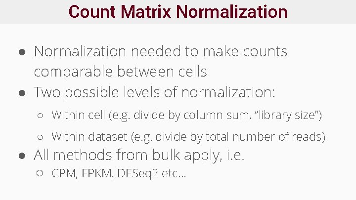
Count Matrix Normalization ● Normalization needed to make counts comparable between cells ● Two possible levels of normalization: ○ Within cell (e. g. divide by column sum, “library size”) ○ Within dataset (e. g. divide by total number of reads) ● All methods from bulk apply, i. e. ○ CPM, FPKM, DESeq 2 etc…

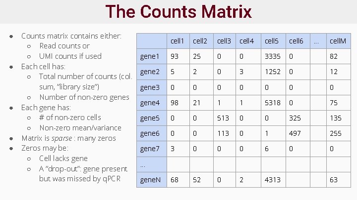
The Counts Matrix ● ● ● Counts matrix contains either: ○ Read counts or ○ UMI counts if used Each cell has: ○ Total number of counts (col. sum, “library size”) ○ Number of non-zero genes Each gene has: ○ # of non-zero cells ○ Non-zero mean/variance Matrix is sparse : many zeros Zeros may be: ○ Cell lacks gene ○ A “drop-out”: gene present but was missed by q. PCR cell 1 cell 2 cell 3 cell 4 cell 5 cell 6 . . . cell. M gene 1 93 25 0 0 3335 0 82 gene 2 5 2 0 3 1252 0 12 gene 3 0 0 0 0 gene 4 98 21 1 1 5318 0 75 gene 5 0 0 513 0 0 325 135 gene 6 0 0 113 0 1 497 255 gene 7 3 0 0 0 68 52 0 2 4313 . . . gene. N 63

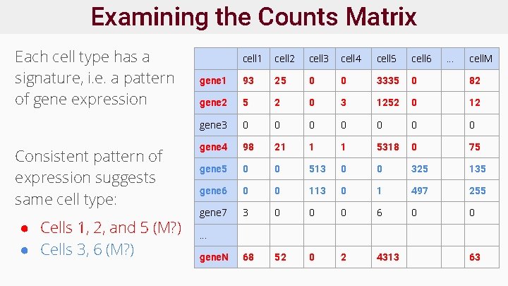
Examining the Counts Matrix Each cell type has a signature, i. e. a pattern of gene expression Consistent pattern of expression suggests same cell type: ● Cells 1, 2, and 5 (M? ) ● Cells 3, 6 (M? ) cell 1 cell 2 cell 3 cell 4 cell 5 cell 6 . . . cell. M gene 1 93 25 0 0 3335 0 82 gene 2 5 2 0 3 1252 0 12 gene 3 0 0 0 0 gene 4 98 21 1 1 5318 0 75 gene 5 0 0 513 0 0 325 135 gene 6 0 0 113 0 1 497 255 gene 7 3 0 0 0 68 52 0 2 4313 . . . gene. N 63

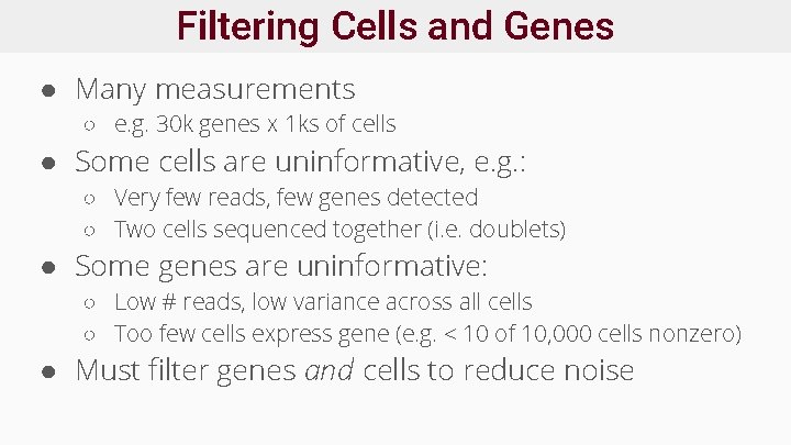
Filtering Cells and Genes ● Many measurements ○ e. g. 30 k genes x 1 ks of cells ● Some cells are uninformative, e. g. : ○ Very few reads, few genes detected ○ Two cells sequenced together (i. e. doublets) ● Some genes are uninformative: ○ Low # reads, low variance across all cells ○ Too few cells express gene (e. g. < 10 of 10, 000 cells nonzero) ● Must filter genes and cells to reduce noise

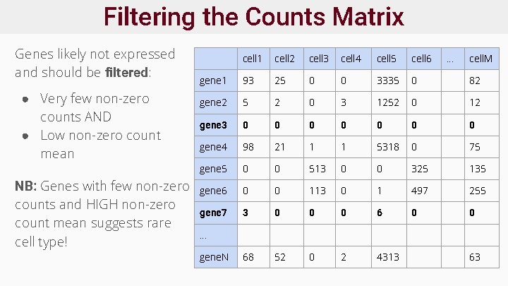
Filtering the Counts Matrix Genes likely not expressed and should be filtered: ● Very few non-zero counts AND ● Low non-zero count mean NB: Genes with few non-zero counts and HIGH non-zero count mean suggests rare cell type! cell 1 cell 2 cell 3 cell 4 cell 5 cell 6 . . . cell. M gene 1 93 25 0 0 3335 0 82 gene 2 5 2 0 3 1252 0 12 gene 3 0 0 0 0 gene 4 98 21 1 1 5318 0 75 gene 5 0 0 513 0 0 325 135 gene 6 0 0 113 0 1 497 255 gene 7 3 0 0 0 68 52 0 2 4313 . . . gene. N 63

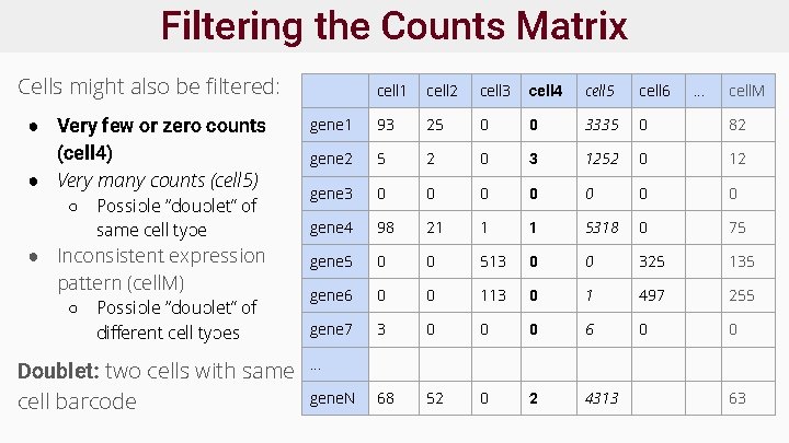
Filtering the Counts Matrix Cells might also be filtered: ● Very few or zero counts (cell 4) ● Very many counts (cell 5) ○ Possible “doublet” of same cell type ● Inconsistent expression pattern (cell. M) ○ Possible “doublet” of different cell types Doublet: two cells with same cell barcode cell 1 cell 2 cell 3 cell 4 cell 5 cell 6 . . . cell. M gene 1 93 25 0 0 3335 0 82 gene 2 5 2 0 3 1252 0 12 gene 3 0 0 0 0 gene 4 98 21 1 1 5318 0 75 gene 5 0 0 513 0 0 325 135 gene 6 0 0 113 0 1 497 255 gene 7 3 0 0 0 68 52 0 2 4313 . . . gene. N 63

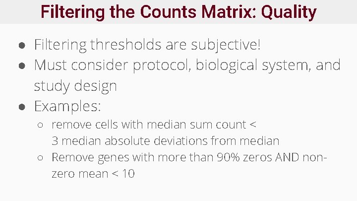
Filtering the Counts Matrix: Quality ● Filtering thresholds are subjective! ● Must consider protocol, biological system, and study design ● Examples: ○ remove cells with median sum count < 3 median absolute deviations from median ○ Remove genes with more than 90% zeros AND nonzero mean < 10

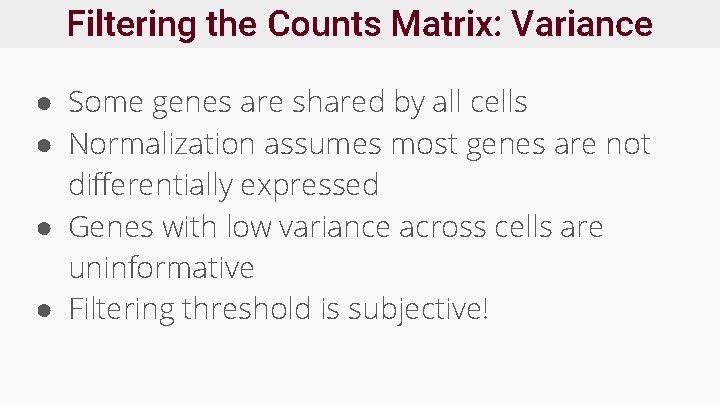
Filtering the Counts Matrix: Variance ● Some genes are shared by all cells ● Normalization assumes most genes are not differentially expressed ● Genes with low variance across cells are uninformative ● Filtering threshold is subjective!

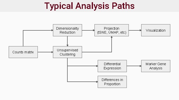
Typical Analysis Paths Dimensionality Reduction Counts matrix Projection (t. SNE, UMAP, etc) Visualization Differential Expression Marker Gene Analysis Unsupervised Clustering Differences in Proportion

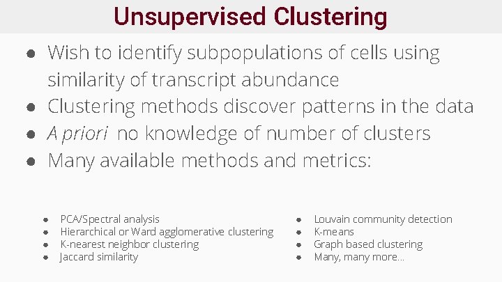
Unsupervised Clustering ● Wish to identify subpopulations of cells using similarity of transcript abundance ● Clustering methods discover patterns in the data ● A priori no knowledge of number of clusters ● Many available methods and metrics: ● ● PCA/Spectral analysis Hierarchical or Ward agglomerative clustering K-nearest neighbor clustering Jaccard similarity ● ● Louvain community detection K-means Graph based clustering Many, many more. . .

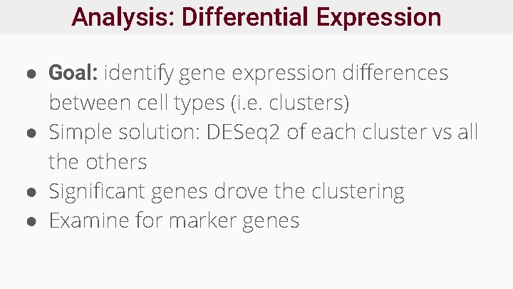
Analysis: Differential Expression ● Goal: identify gene expression differences between cell types (i. e. clusters) ● Simple solution: DESeq 2 of each cluster vs all the others ● Significant genes drove the clustering ● Examine for marker genes

Marker Gene Analysis ● Goal: Label each cluster to known cell type ● Biological domain experts know which genes are expressed by each cell type ● Some clusters may be difficult to label (novel cell types? ) ● NB: cells of one cell type may cluster by state , e. g. cell cycle phase G 1

Dimensionality Reduction ● Counts matrix may have many dimensions ○ 1000 s of genes x 1000 s of cells ● Reduces # dimensions while preserving variance ● May be necessary for large datasets (>1 M cells) to make downstream analysis algorithms tractable ● Many methods available, including: ○ PCA ○ Multidimensional Scaling (MDS) ○ Downsampling

Projection + Visualization ● Goal: accurately visualize cell clusters in two dimensions ● Projection: embed samples of high dimensional space into lower dimensional space, retaining structure of data ○ e. g. map from (1000 s genes x 1000 s cells) to 2 (i. e. <x, y>) ● Ideally preserve both local and global structure ● NB: this is challenging to do efficiently+accurately! ● Available methods: ○ t-SNE: t-statistic Stochastic Neighbor Embedding ○ UMAP: Uniform Manifold Approx. and Mapping ○ PCA

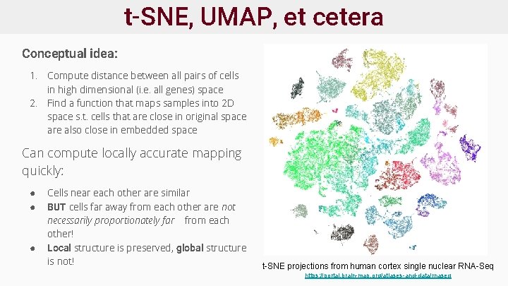
t-SNE, UMAP, et cetera Conceptual idea: 1. Compute distance between all pairs of cells in high dimensional (i. e. all genes) space 2. Find a function that maps samples into 2 D space s. t. cells that are close in original space are also close in embedded space Can compute locally accurate mapping quickly: ● ● ● Cells near each other are similar BUT cells far away from each other are not necessarily proportionately far from each other! Local structure is preserved, global structure is not! t-SNE projections from human cortex single nuclear RNA-Seq https: //portal. brain-map. org/atlases-and-data/rnaseq

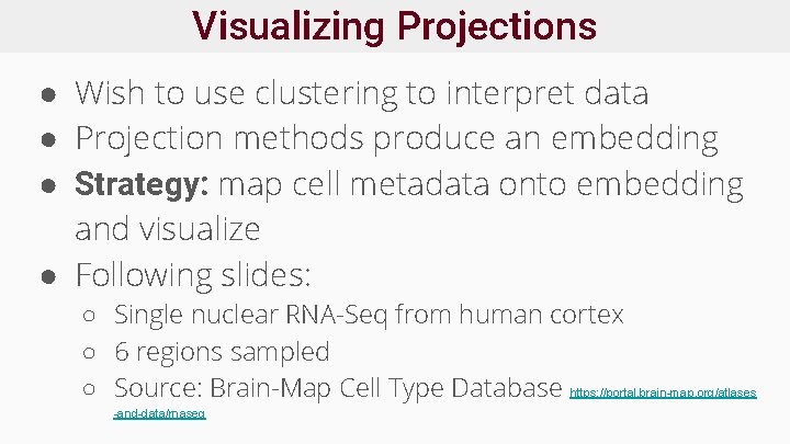
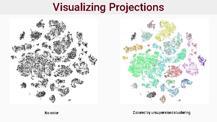
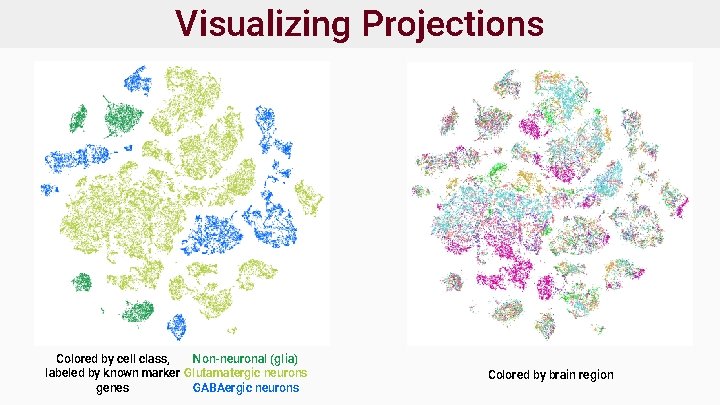
Visualizing Projections ● Wish to use clustering to interpret data ● Projection methods produce an embedding ● Strategy: map cell metadata onto embedding and visualize ● Following slides: ○ Single nuclear RNA-Seq from human cortex ○ 6 regions sampled ○ Source: Brain-Map Cell Type Database https: //portal. brain-map. org/atlases -and-data/rnaseq

Visualizing Projections No color Colored by unsupervised clustering

Visualizing Projections Colored by cell class, Non-neuronal (glia) labeled by known marker Glutamatergic neurons genes GABAergic neurons Colored by brain region

The Many Subjects We Didn’t Cover ● Supervised clustering of cells by known markers/cell states (e. g. cell cycle) ● Comparing different samples ● Pseudotime Analysis ○ Inferring cellular development/change over time ● Imputation ○ Infer expression values for “dropout” genes ● Many more. . .

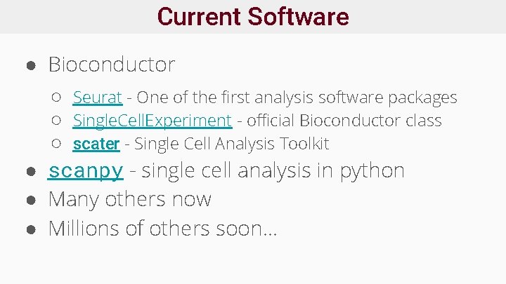
Current Software ● Bioconductor ○ Seurat - One of the first analysis software packages ○ Single. Cell. Experiment - official Bioconductor class ○ scater - Single Cell Analysis Toolkit ● scanpy - single cell analysis in python ● Many others now ● Millions of others soon. . .