Simultaneous Segmentation and 3 D Pose Estimation of

Simultaneous Segmentation and 3 D Pose Estimation of Humans Philip H. S. Torr Pawan Kumar, Pushmeet Kohli, Matt Bray Oxford Brookes University Arasanathan Thayananthan, Bjorn Stenger, Roberto Cipolla Cambridge University

Algebra n Unifying Conjecture Tracking = Detection = Recognition n Detection = Segmentation n • therefore n Tracking (pose estimation)=Segmentation?

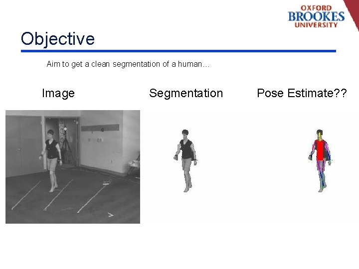
Objective Aim to get a clean segmentation of a human… Image Segmentation Pose Estimate? ?

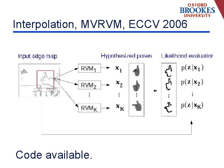
Developments n n n ICCV 2003, pose estimation as fast nearest neighbour plus dynamics (inspired by Gavrilla and Toyoma & Blake) BMVC 2004, parts based chamfer to make space of templates more flexible (a la pictorial structures of Huttenlocher) CVPR 2005, Obj. Cut combining segmentation and detection. ICCV 2005 Dynamic Graph Cuts ECCV 2006, interpolation of poses using the MVRVM (Agarwal and Triggs) ECCV 2006 combination of pose estimation and segmentation using graph cuts.

Tracking as Detection (Stenger et al ICCV 2003) Detection has become very efficient, e. g. real-time face detection, pedestrian detection Example: Pedestrian detection [Gavrila & Philomin, 1999]: n Find match among large number of exemplar templates Issues: n Number of templates needed n Efficient search n Robust cost function

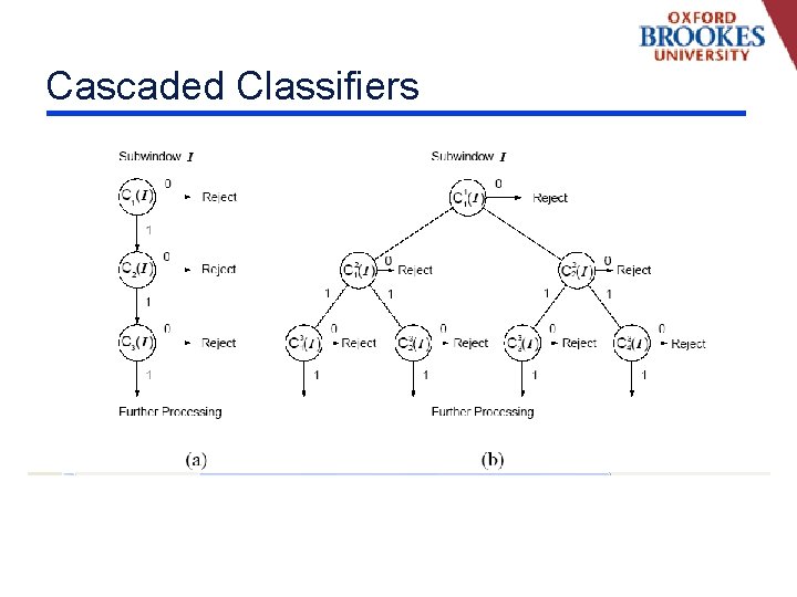
Cascaded Classifiers

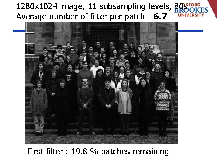
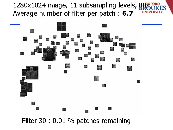
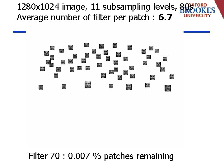
1280 x 1024 image, 11 subsampling levels, 80 s Average number of filter patch : 6. 7 First filter : 19. 8 % patches remaining

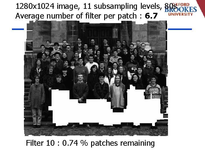
1280 x 1024 image, 11 subsampling levels, 80 s Average number of filter patch : 6. 7 Filter 10 : 0. 74 % patches remaining

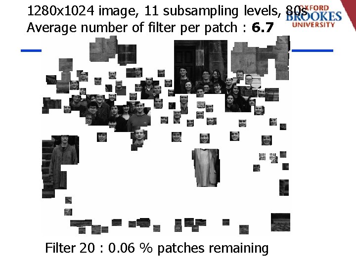
1280 x 1024 image, 11 subsampling levels, 80 s Average number of filter patch : 6. 7 Filter 20 : 0. 06 % patches remaining

1280 x 1024 image, 11 subsampling levels, 80 s Average number of filter patch : 6. 7 Filter 30 : 0. 01 % patches remaining

1280 x 1024 image, 11 subsampling levels, 80 s Average number of filter patch : 6. 7 Filter 70 : 0. 007 % patches remaining

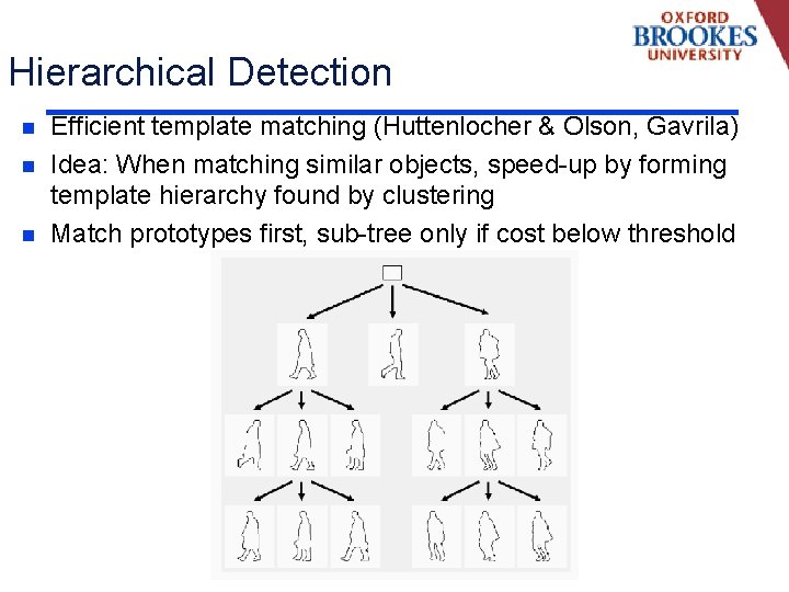
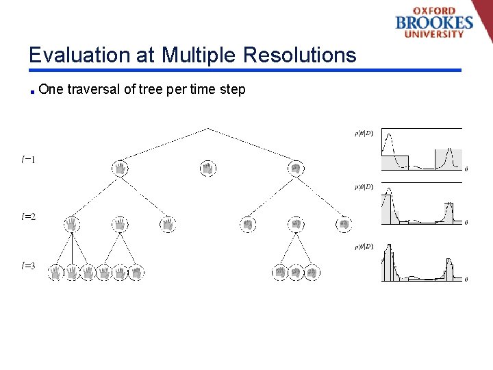
Hierarchical Detection n Efficient template matching (Huttenlocher & Olson, Gavrila) Idea: When matching similar objects, speed-up by forming template hierarchy found by clustering Match prototypes first, sub-tree only if cost below threshold

Trees n These search trees are the same as used for efficient nearest neighbour. n Add dynamic model and • Detection = Tracking = Recognition

Evaluation at Multiple Resolutions One traversal of tree per time step

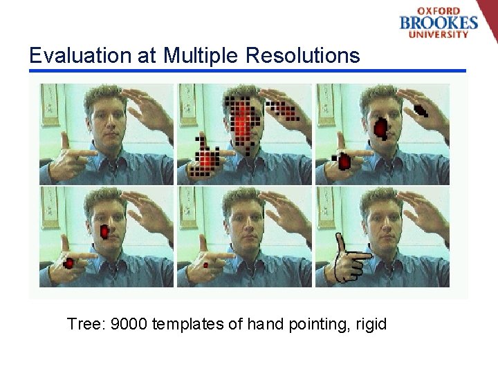
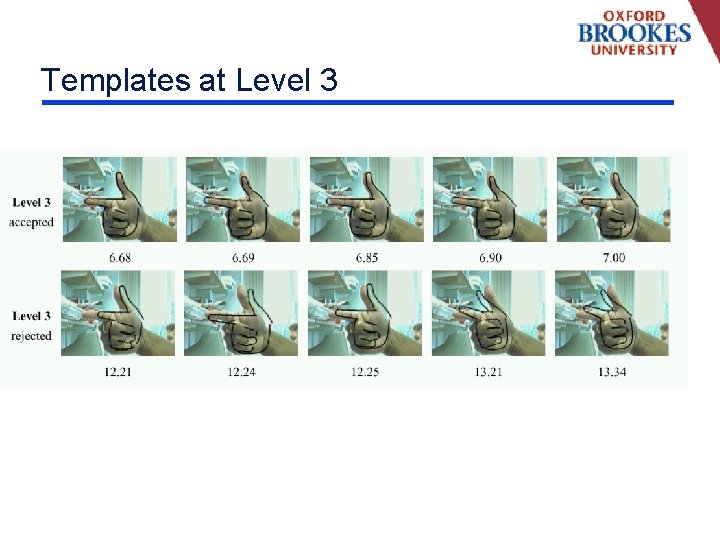
Evaluation at Multiple Resolutions Tree: 9000 templates of hand pointing, rigid

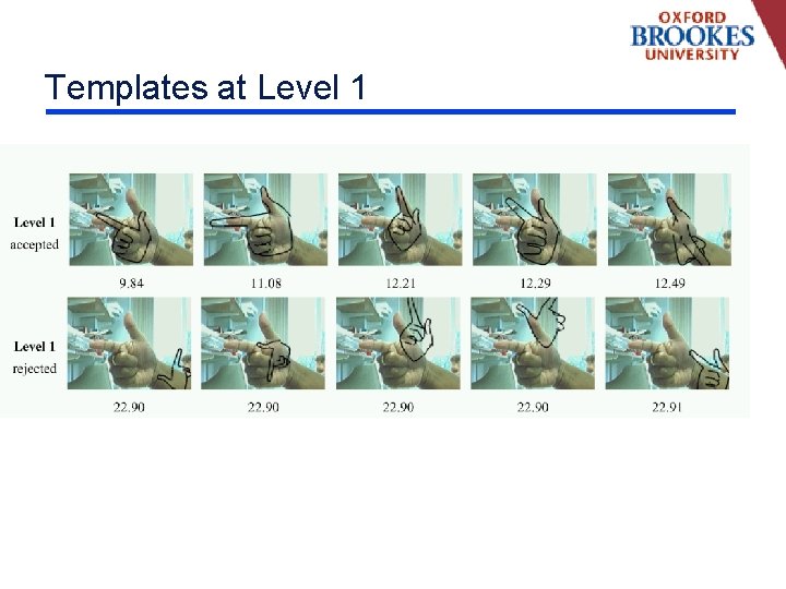
Templates at Level 1

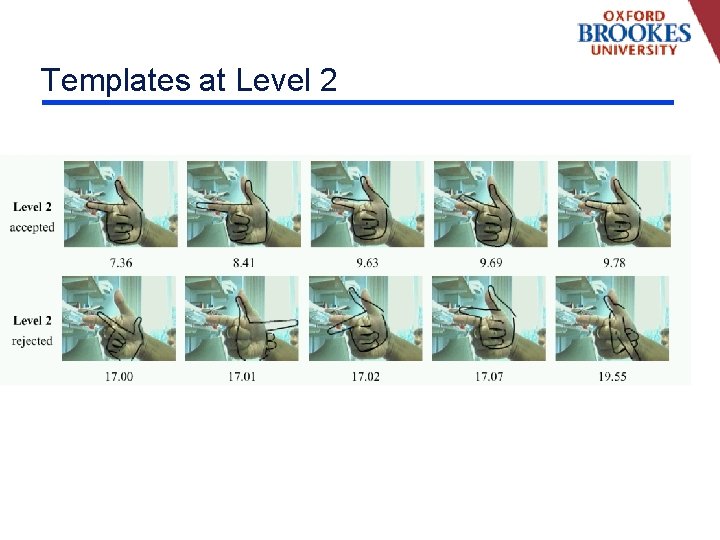
Templates at Level 2

Templates at Level 3

Comparison with Particle Filters n This method is grid based, • No need to render the model on line • Like efficient search • Can always use this as a proposal process for a particle filter if need be.

Interpolation, MVRVM, ECCV 2006 Code available.

Energy being Optimized, link to graph cuts n Combination of • Edge term (quickly evaluated using chamfer) • Interior term (quickly evaluated using integral images) n Note that possible templates are a bit like cuts that we put down, one could think of this whole process as a constrained search for the best graph cut.

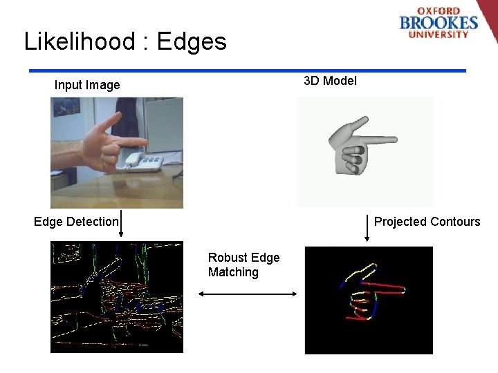
Likelihood : Edges 3 D Model Input Image Edge Detection Projected Contours Robust Edge Matching

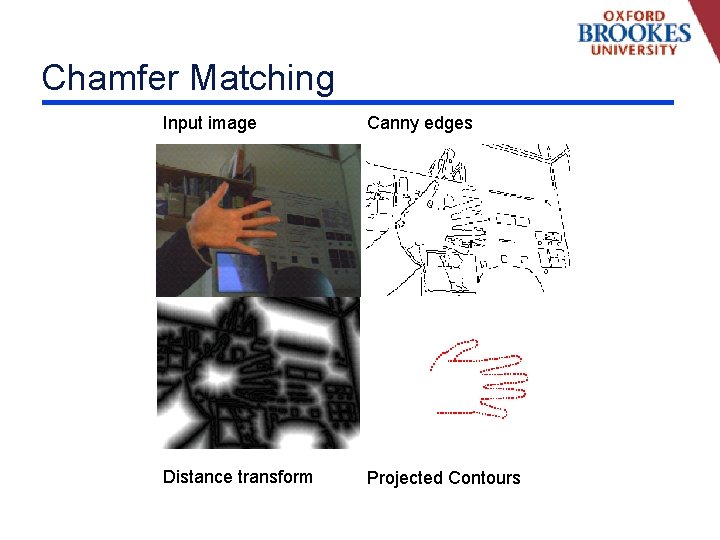
Chamfer Matching Input image Canny edges Distance transform Projected Contours

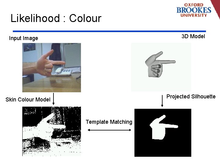
Likelihood : Colour 3 D Model Input Image Projected Silhouette Skin Colour Model Template Matching

Template Matching = n Template Matching = constrained search for a cut/segmentation? n Detection = Segmentation?

Objective Aim to get a clean segmentation of a human… Image Segmentation Pose Estimate? ?

MRF for Interactive Image Segmentation, Boykov and Jolly [ICCV 2001] Energy. MRF = Unary likelihood Contrast Term Uniform Prior (Potts Model) Maximum-a-posteriori (MAP) solution x* = arg min E(x) x Data (D) Unary likelihood Pair-wise Terms MAP Solution

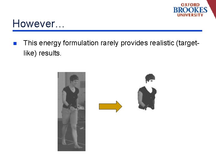
However… n This energy formulation rarely provides realistic (targetlike) results.

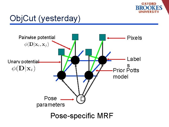
Obj. Cut (yesterday) Pixels Pairwise potential Label s Prior Potts model Unary potential Pose parameters � Pose-specific MRF

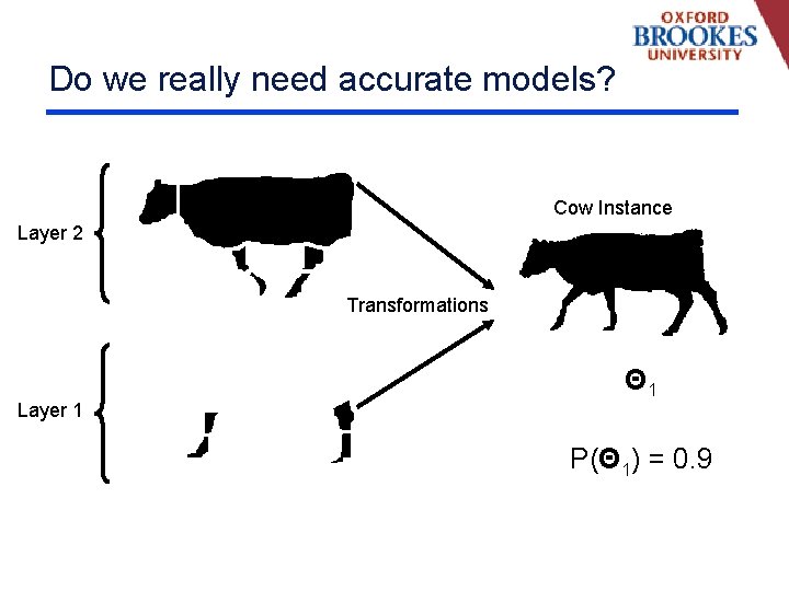
Do we really need accurate models? Cow Instance Layer 2 Transformations Layer 1 Θ 1 P(Θ 1) = 0. 9

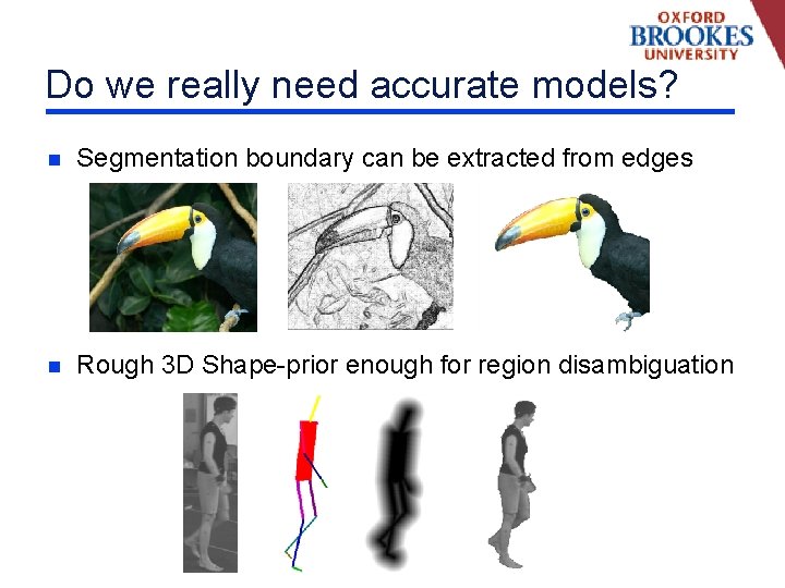
Do we really need accurate models? n Segmentation boundary can be extracted from edges n Rough 3 D Shape-prior enough for region disambiguation

Energy of the Pose-specific MRF Energy to be minimized Pairwise potential Unary term Potts model Shape prior But what should be the value of θ?

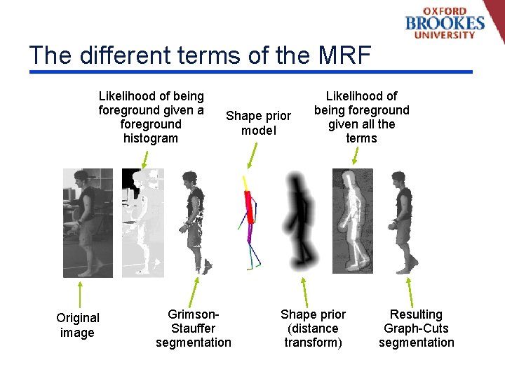
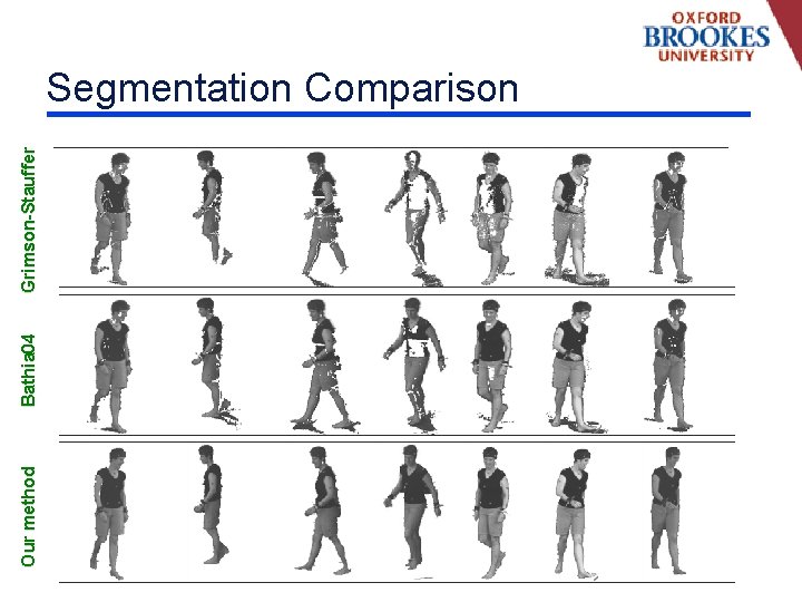
The different terms of the MRF Likelihood of being foreground given a foreground histogram Original image Shape prior model Grimson. Stauffer segmentation Likelihood of being foreground given all the terms Shape prior (distance transform) Resulting Graph-Cuts segmentation

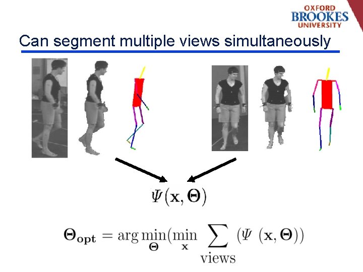
Can segment multiple views simultaneously

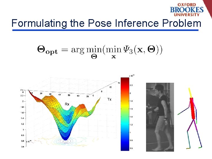
Solve via gradient descent n Comparable to level set methods n Could use other approaches (e. g. Objcut) n Need a graph cut per function evaluation

Formulating the Pose Inference Problem

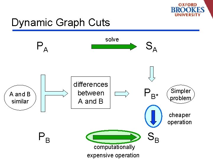
But… … to compute the MAP of E(x) w. r. t the pose, it means that the unary terms will be changed at EACH iteration and the maxflow recomputed! However… n Kohli and Torr showed how dynamic graph cuts can be used to efficiently find MAP solutions for MRFs that change minimally from one time instant to the next: Dynamic Graph Cuts (ICCV 05).

Dynamic Graph Cuts PA solve differences between A and B similar SA PB* Simpler problem cheaper operation PB computationally expensive operation SB

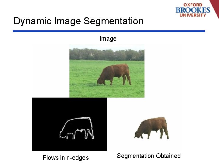
Dynamic Image Segmentation Image Flows in n-edges Segmentation Obtained

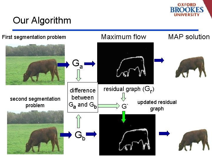
Our Algorithm Maximum flow First segmentation problem MAP solution Ga second segmentation problem difference between Ga and Gb Gb residual graph (Gr) G` updated residual graph

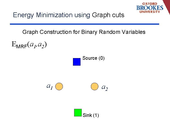
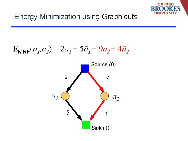
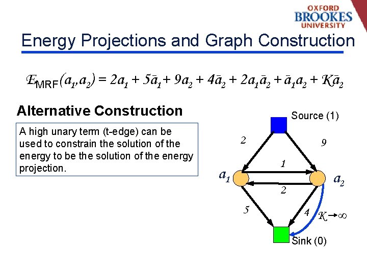
Energy Minimization using Graph cuts Graph Construction for Binary Random Variables EMRF(a 1, a 2) Source (0) a 1 a 2 Sink (1)

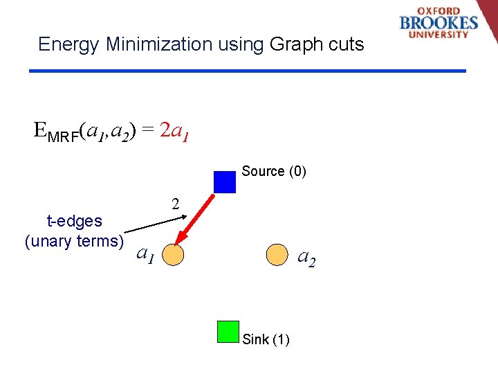
Energy Minimization using Graph cuts EMRF(a 1, a 2) = 2 a 1 Source (0) t-edges (unary terms) 2 a 1 a 2 Sink (1)

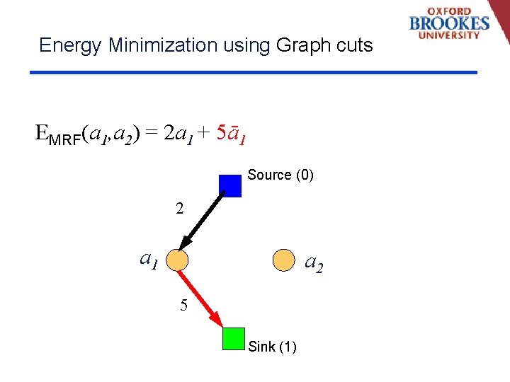
Energy Minimization using Graph cuts EMRF(a 1, a 2) = 2 a 1 + 5ā1 Source (0) 2 a 1 a 2 5 Sink (1)

Energy Minimization using Graph cuts EMRF(a 1, a 2) = 2 a 1 + 5ā1+ 9 a 2 + 4ā2 Source (0) 2 9 a 1 a 2 5 4 Sink (1)

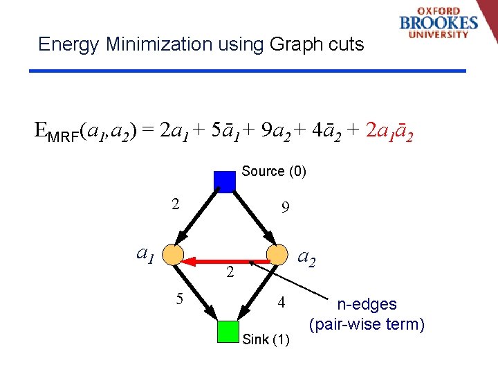
Energy Minimization using Graph cuts EMRF(a 1, a 2) = 2 a 1 + 5ā1+ 9 a 2 + 4ā2 + 2 a 1ā2 Source (0) 2 a 1 9 a 2 2 5 4 Sink (1) n-edges (pair-wise term)

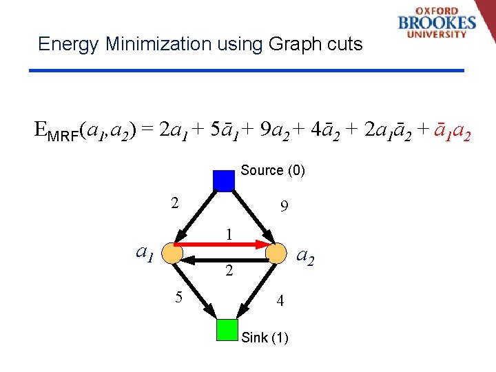
Energy Minimization using Graph cuts EMRF(a 1, a 2) = 2 a 1 + 5ā1+ 9 a 2 + 4ā2 + 2 a 1ā2 + ā1 a 2 Source (0) 2 9 1 a 2 2 5 4 Sink (1)

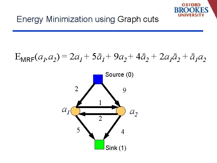
Energy Minimization using Graph cuts EMRF(a 1, a 2) = 2 a 1 + 5ā1+ 9 a 2 + 4ā2 + 2 a 1ā2 + ā1 a 2 Source (0) 2 9 1 a 2 2 5 4 Sink (1)

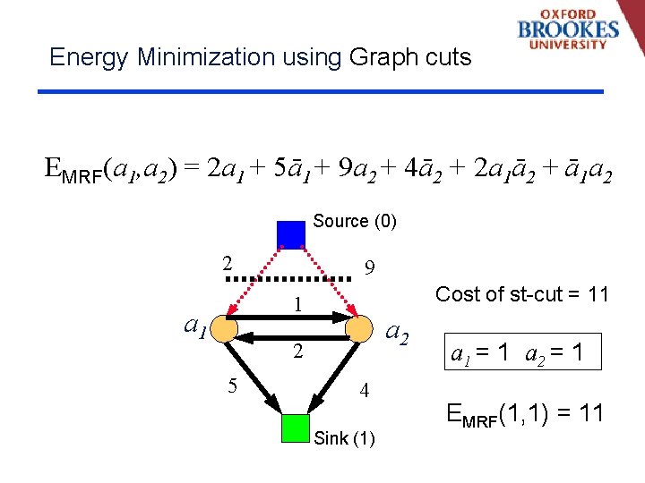
Energy Minimization using Graph cuts EMRF(a 1, a 2) = 2 a 1 + 5ā1+ 9 a 2 + 4ā2 + 2 a 1ā2 + ā1 a 2 Source (0) 2 9 Cost of st-cut = 11 1 a 2 2 5 4 Sink (1) a 1 = 1 a 2 = 1 EMRF(1, 1) = 11

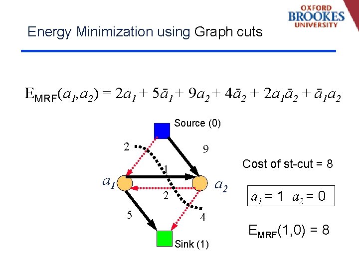
Energy Minimization using Graph cuts EMRF(a 1, a 2) = 2 a 1 + 5ā1+ 9 a 2 + 4ā2 + 2 a 1ā2 + ā1 a 2 Source (0) 2 9 Cost of st-cut = 8 1 a 2 2 5 4 Sink (1) a 1 = 1 a 2 = 0 EMRF(1, 0) = 8

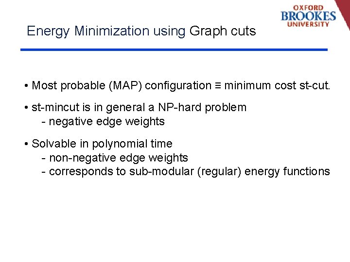
Energy Minimization using Graph cuts • Most probable (MAP) configuration ≡ minimum cost st-cut. • st-mincut is in general a NP-hard problem - negative edge weights • Solvable in polynomial time - non-negative edge weights - corresponds to sub-modular (regular) energy functions

Computing the st-mincut from Max-flow algorithms • The Max-flow Problem - Edge capacity and flow balance constraints • Notation - Residual capacity (edge capacity – current flow) - Augmenting path Source (0) 2 1 a 1 • Simple Augmenting Path based Algorithms - Repeatedly find augmenting paths and push flow. - Saturated edges constitute the st-mincut. [Ford-Fulkerson Theorem] 9 a 2 2 5 4 Sink (1)

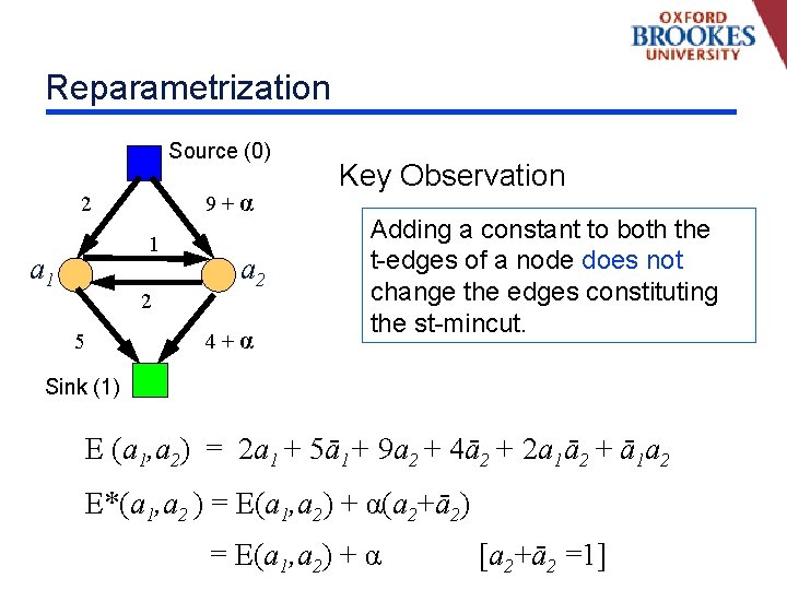
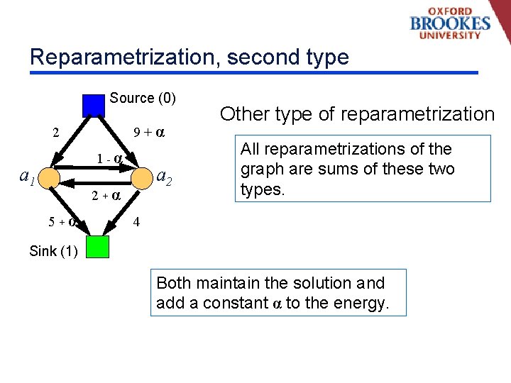
Reparametrization Source (0) 9+α 2 1 a 1 2 5 a 2 4+α Key Observation Adding a constant to both the t-edges of a node does not change the edges constituting the st-mincut. Sink (1) E (a 1, a 2) = 2 a 1 + 5ā1+ 9 a 2 + 4ā2 + 2 a 1ā2 + ā1 a 2 E*(a 1, a 2 ) = E(a 1, a 2) + α(a 2+ā2) = E(a 1, a 2) + α [a 2+ā2 =1]

Reparametrization, second type Source (0) 9+α 2 1 -α a 1 a 2 2+α 5+α Other type of reparametrization All reparametrizations of the graph are sums of these two types. 4 Sink (1) Both maintain the solution and add a constant α to the energy.

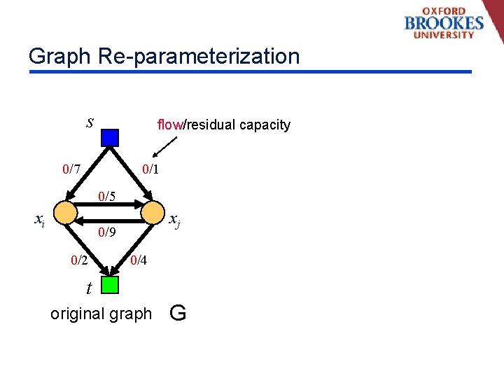
Graph Re-parameterization s flow/residual capacity 0/7 0/1 0/5 xi xj 0/9 0/2 0/4 t original graph G

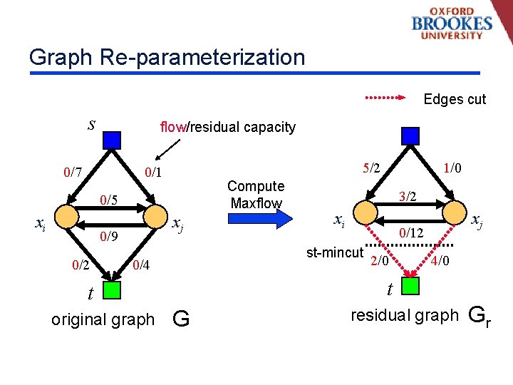
Graph Re-parameterization Edges cut s flow/residual capacity 0/7 5/2 0/1 Compute Maxflow 0/5 xi xj 0/9 0/2 xi xj 0/12 2/0 4/0 t t original graph 3/2 st-mincut 0/4 1/0 G residual graph Gr

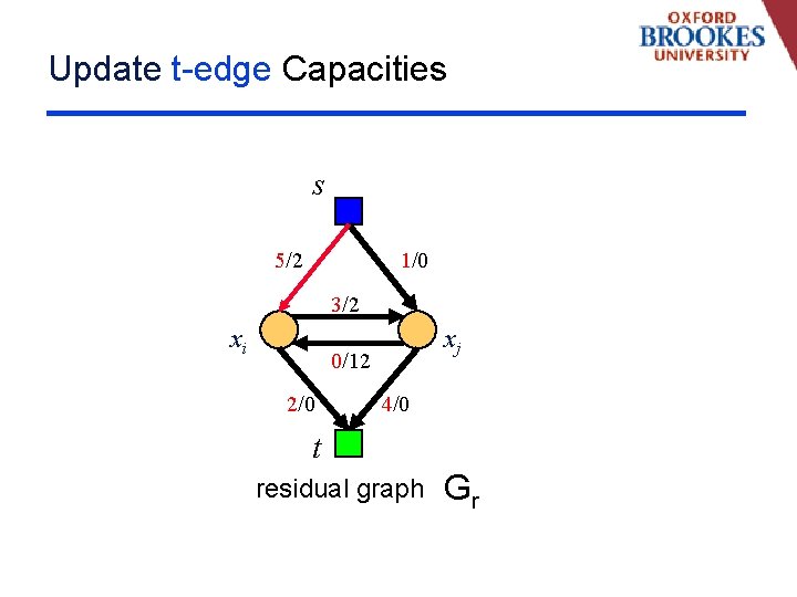
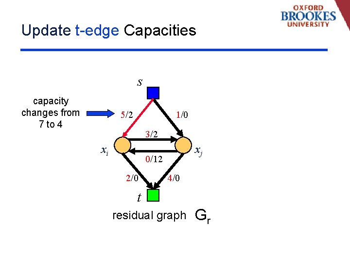
Update t-edge Capacities s 5/2 1/0 3/2 xi xj 0/12 2/0 4/0 t residual graph Gr

Update t-edge Capacities s capacity changes from 7 to 4 5/2 1/0 3/2 xi xj 0/12 2/0 4/0 t residual graph Gr

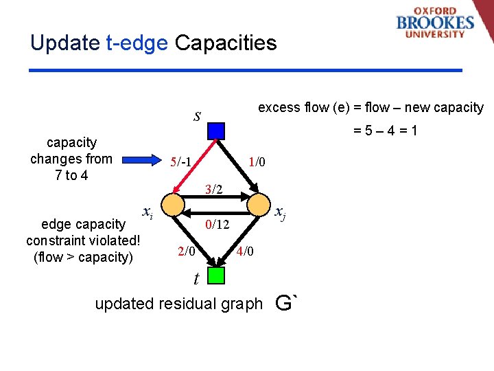
Update t-edge Capacities excess flow (e) = flow – new capacity s capacity changes from 7 to 4 edge capacity constraint violated! (flow > capacity) =5– 4=1 5/-1 1/0 3/2 xi xj 0/12 2/0 4/0 t updated residual graph G`

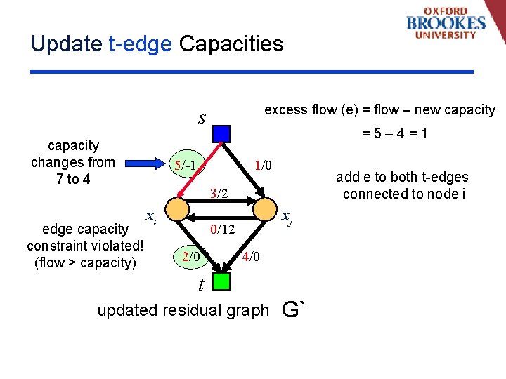
Update t-edge Capacities excess flow (e) = flow – new capacity s capacity changes from 7 to 4 edge capacity constraint violated! (flow > capacity) =5– 4=1 5/-1 1/0 add e to both t-edges connected to node i 3/2 xi xj 0/12 2/0 4/0 t updated residual graph G`

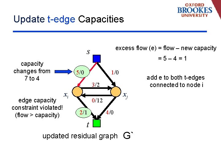
Update t-edge Capacities excess flow (e) = flow – new capacity s capacity changes from 7 to 4 edge capacity constraint violated! (flow > capacity) =5– 4=1 5/0 1/0 add e to both t-edges connected to node i 3/2 xi xj 0/12 2/1 4/0 t updated residual graph G`

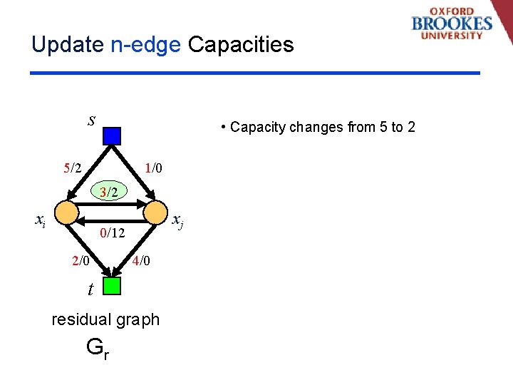
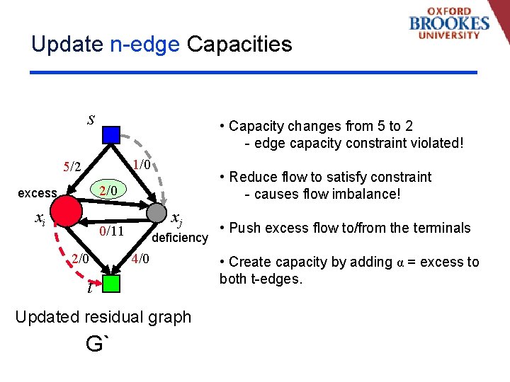
Update n-edge Capacities s • Capacity changes from 5 to 2 5/2 1/0 3/2 xi xj 0/12 2/0 4/0 t residual graph Gr

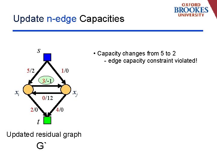
Update n-edge Capacities s • Capacity changes from 5 to 2 - edge capacity constraint violated! 5/2 1/0 3/-1 xi xj 0/12 2/0 4/0 t Updated residual graph G`

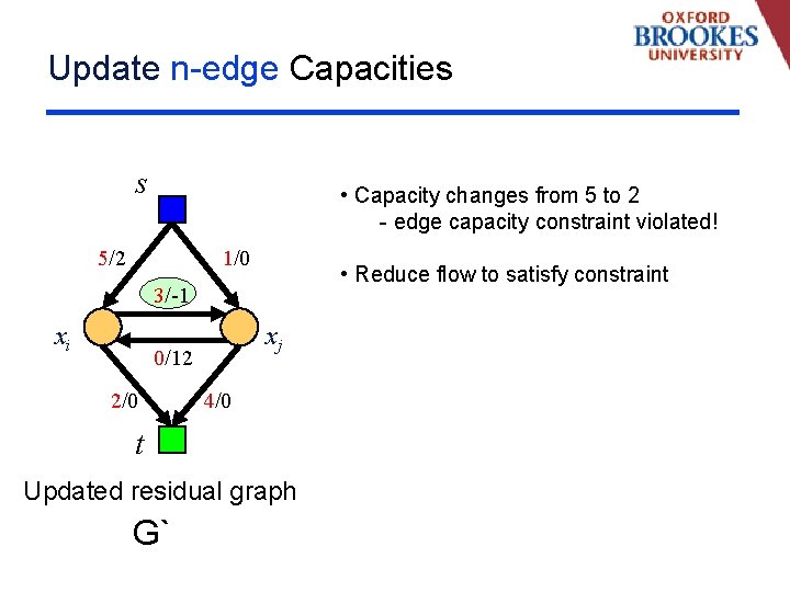
Update n-edge Capacities s • Capacity changes from 5 to 2 - edge capacity constraint violated! 5/2 1/0 • Reduce flow to satisfy constraint 3/-1 xi xj 0/12 2/0 4/0 t Updated residual graph G`

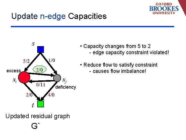
Update n-edge Capacities s • Capacity changes from 5 to 2 - edge capacity constraint violated! 1/0 5/2 • Reduce flow to satisfy constraint - causes flow imbalance! 2/0 excess xi xj 0/11 2/0 deficiency 4/0 t Updated residual graph G`

Update n-edge Capacities s • Capacity changes from 5 to 2 - edge capacity constraint violated! 1/0 5/2 • Reduce flow to satisfy constraint - causes flow imbalance! 2/0 excess xi xj 0/11 2/0 deficiency 4/0 t Updated residual graph G` • Push excess flow to/from the terminals • Create capacity by adding α = excess to both t-edges.

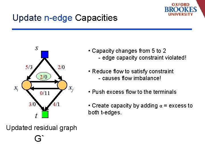
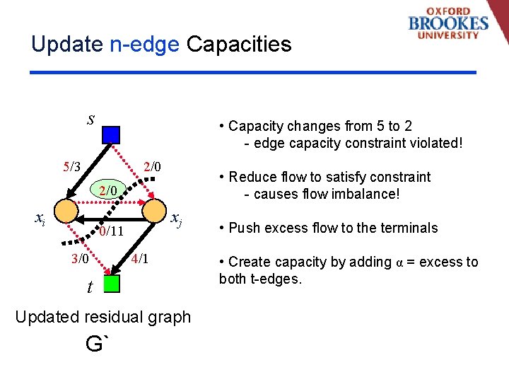
Update n-edge Capacities s • Capacity changes from 5 to 2 - edge capacity constraint violated! 5/3 2/0 • Reduce flow to satisfy constraint - causes flow imbalance! 2/0 xi xj 0/11 3/0 4/1 t Updated residual graph G` • Push excess flow to the terminals • Create capacity by adding α = excess to both t-edges.

Update n-edge Capacities s • Capacity changes from 5 to 2 - edge capacity constraint violated! 5/3 2/0 • Reduce flow to satisfy constraint - causes flow imbalance! 2/0 xi xj 0/11 3/0 4/1 t Updated residual graph G` • Push excess flow to the terminals • Create capacity by adding α = excess to both t-edges.

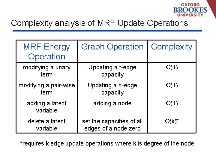
Complexity analysis of MRF Update Operations MRF Energy Operation Graph Operation Complexity modifying a unary term Updating a t-edge capacity O(1) modifying a pair-wise term Updating a n-edge capacity O(1) adding a latent variable adding a node O(1) delete a latent variable set the capacities of all edges of a node zero O(k)* *requires k edge update operations where k is degree of the node

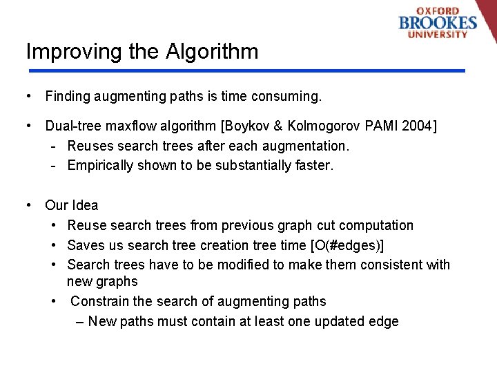
Improving the Algorithm • Finding augmenting paths is time consuming. • Dual-tree maxflow algorithm [Boykov & Kolmogorov PAMI 2004] - Reuses search trees after each augmentation. - Empirically shown to be substantially faster. • Our Idea • Reuse search trees from previous graph cut computation • Saves us search tree creation tree time [O(#edges)] • Search trees have to be modified to make them consistent with new graphs • Constrain the search of augmenting paths – New paths must contain at least one updated edge

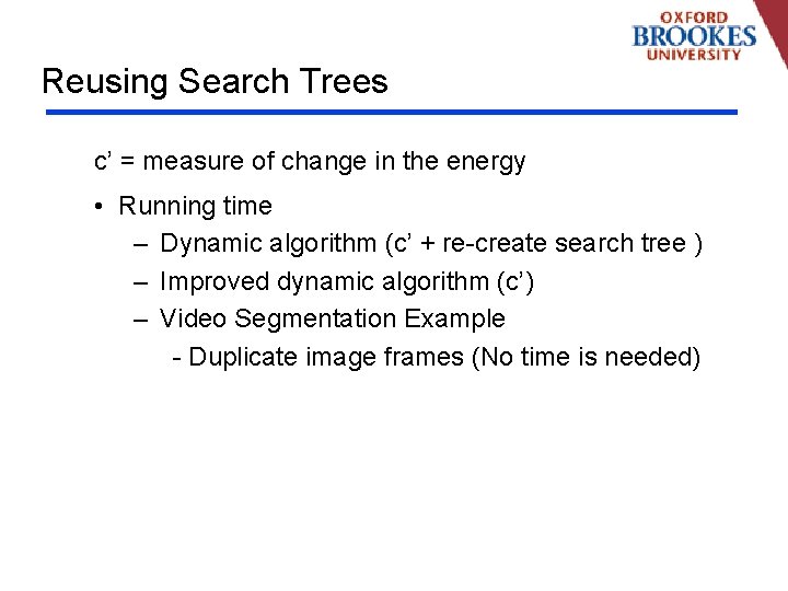
Reusing Search Trees c’ = measure of change in the energy • Running time – Dynamic algorithm (c’ + re-create search tree ) – Improved dynamic algorithm (c’) – Video Segmentation Example - Duplicate image frames (No time is needed)

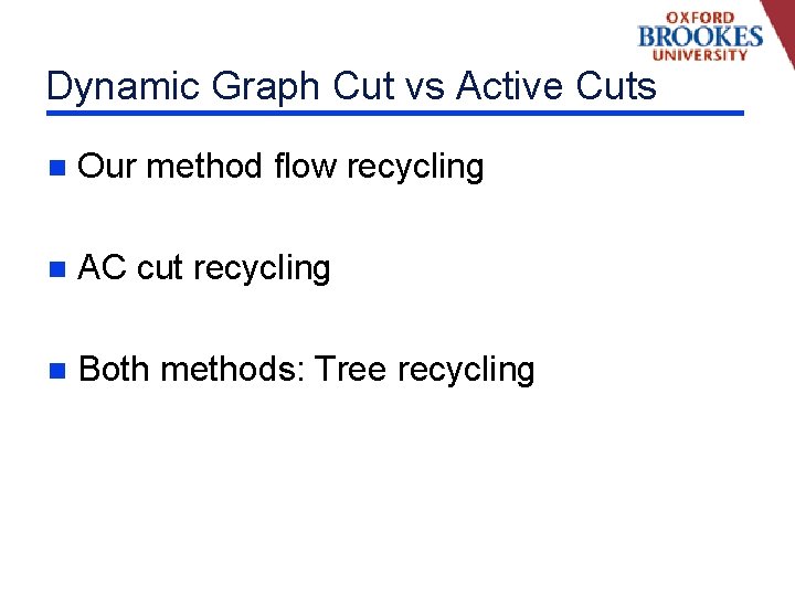
Dynamic Graph Cut vs Active Cuts n Our method flow recycling n AC cut recycling n Both methods: Tree recycling

Experimental Analysis • Compared results with the best static algorithm. - Dual-tree algorithm [Boykov & Kolmogorov PAMI 2004] • Applications - Interactive Image Segmentation - Image Segmentation in Videos

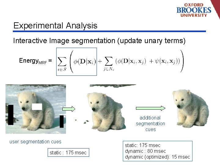
Experimental Analysis Interactive Image segmentation (update unary terms) Energy. MRF = additional segmentation cues user segmentation cues static : 175 msec static: 175 msec dynamic : 80 msec dynamic (optimized): 15 msec

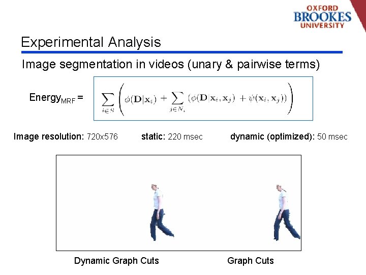
Experimental Analysis Image segmentation in videos (unary & pairwise terms) Energy. MRF = Image resolution: 720 x 576 static: 220 msec Dynamic Graph Cuts dynamic (optimized): 50 msec Graph Cuts

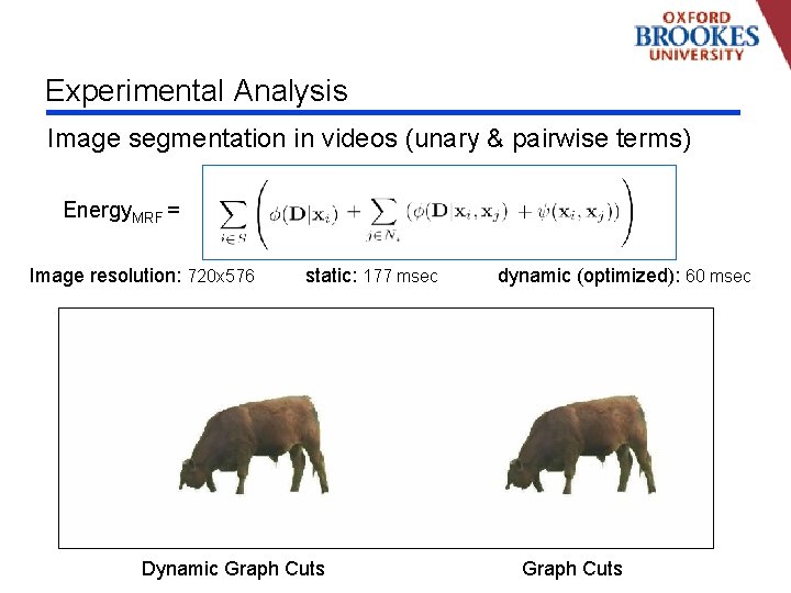
Experimental Analysis Image segmentation in videos (unary & pairwise terms) Energy. MRF = Image resolution: 720 x 576 static: 177 msec Dynamic Graph Cuts dynamic (optimized): 60 msec Graph Cuts

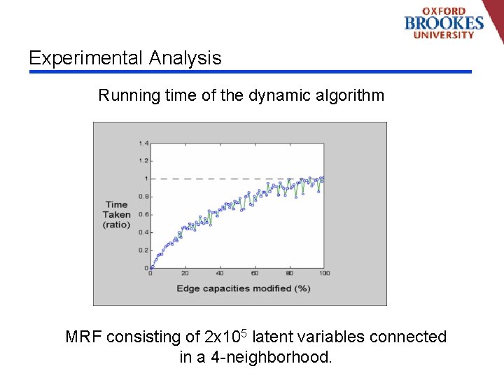
Experimental Analysis Running time of the dynamic algorithm MRF consisting of 2 x 105 latent variables connected in a 4 -neighborhood.

Other uses n Can be used to compute uncertainty in graph cuts via max marginals. n Max marginals can be used for parameter learning in MRF’s.

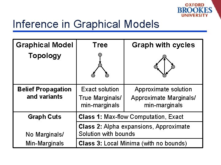
Inference in Graphical Models Graphical Model Topology Tree Graph with cycles Belief Propagation and variants Exact solution True Marginals/ min-marginals Approximate solution Approximate Marginals/ min-marginals Graph Cuts No Marginals/ Min-Marginals Class 1: Max-flow Computation, Exact Class 2: Alpha expansions, Approximate Solution with bounds Class 3: Local Minima (with no bounds)

Inference in Graphical Models Min-Marginals Energies(ψ) - Minimize joint energy over all other variables. - Related to max-marginals as: µj = (1/z)*exp(-ψj) - Can be used to compute confidence as: σj = µ j / Σa µa = exp(-ψi) / Σa exp(-ψa)

Energy Projections and Graph Construction EMRF(a 1, a 2) = 2 a 1 + 5ā1+ 9 a 2 + 4ā2 + 2 a 1ā2 + ā1 a 2 + Kā2 Alternative Construction A high unary term (t-edge) can be used to constrain the solution of the energy to be the solution of the energy projection. Source (1) 2 9 1 a 2 2 5 4 K ∞ Sink (0)

Our method Bathia 04 Grimson-Stauffer Segmentation Comparison

Face Detector and Obj. Cut

Segmentation

Segmentation

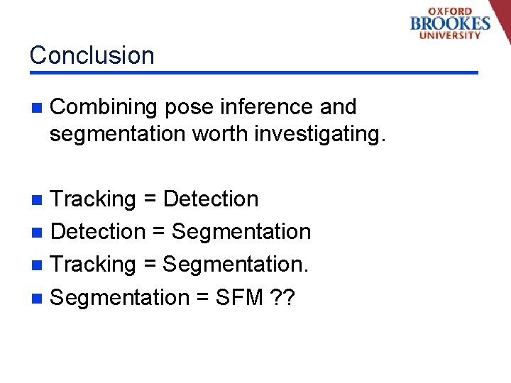
Conclusion n Combining pose inference and segmentation worth investigating. Tracking = Detection n Detection = Segmentation n Tracking = Segmentation. n Segmentation = SFM ? ? n