Simultaneous Segmentation and 3 D Pose Estimation of

Simultaneous Segmentation and 3 D Pose Estimation of Humans or Detection + Segmentation = Tracking? Philip H. S. Torr Pawan Kumar, Pushmeet Kohli, Matt Bray Oxford Brookes University Andrew Zisserman Oxford Arasanathan Thayananthan, Bjorn Stenger, Roberto Cipolla Cambridge

Algebra n Unifying Conjecture Tracking = Detection = Recognition n Detection = Segmentation n • therefore n Tracking (pose estimation)=Segmentation?

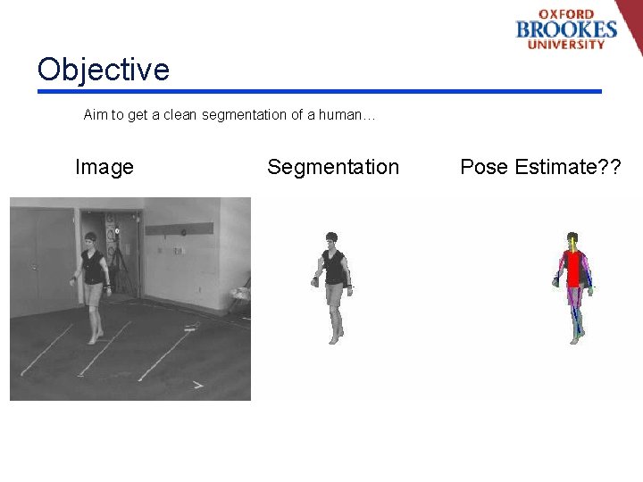
Objective Aim to get a clean segmentation of a human… Image Segmentation Pose Estimate? ?

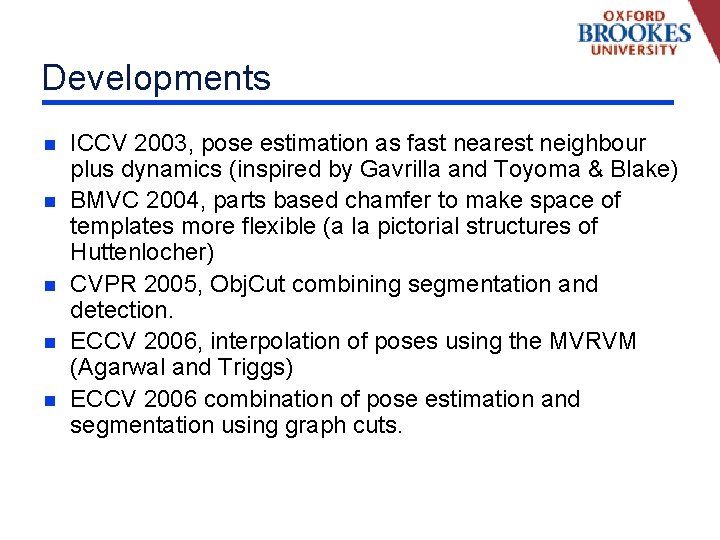
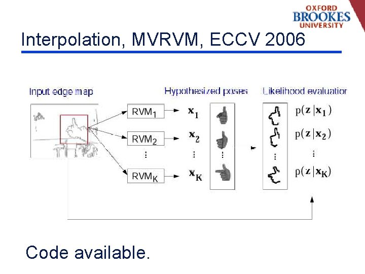
Developments n n n ICCV 2003, pose estimation as fast nearest neighbour plus dynamics (inspired by Gavrilla and Toyoma & Blake) BMVC 2004, parts based chamfer to make space of templates more flexible (a la pictorial structures of Huttenlocher) CVPR 2005, Obj. Cut combining segmentation and detection. ECCV 2006, interpolation of poses using the MVRVM (Agarwal and Triggs) ECCV 2006 combination of pose estimation and segmentation using graph cuts.

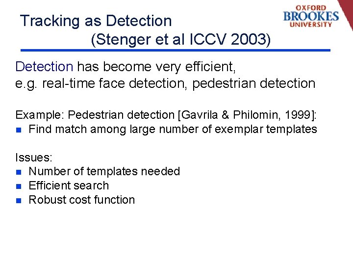
Tracking as Detection (Stenger et al ICCV 2003) Detection has become very efficient, e. g. real-time face detection, pedestrian detection Example: Pedestrian detection [Gavrila & Philomin, 1999]: n Find match among large number of exemplar templates Issues: n Number of templates needed n Efficient search n Robust cost function

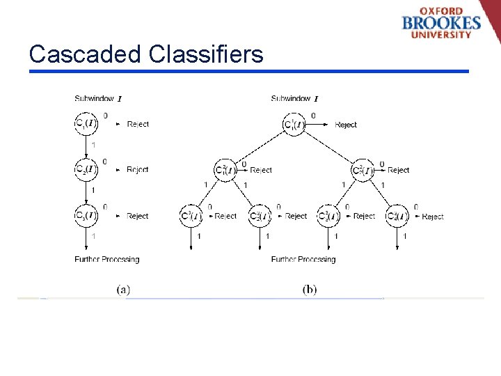
Cascaded Classifiers

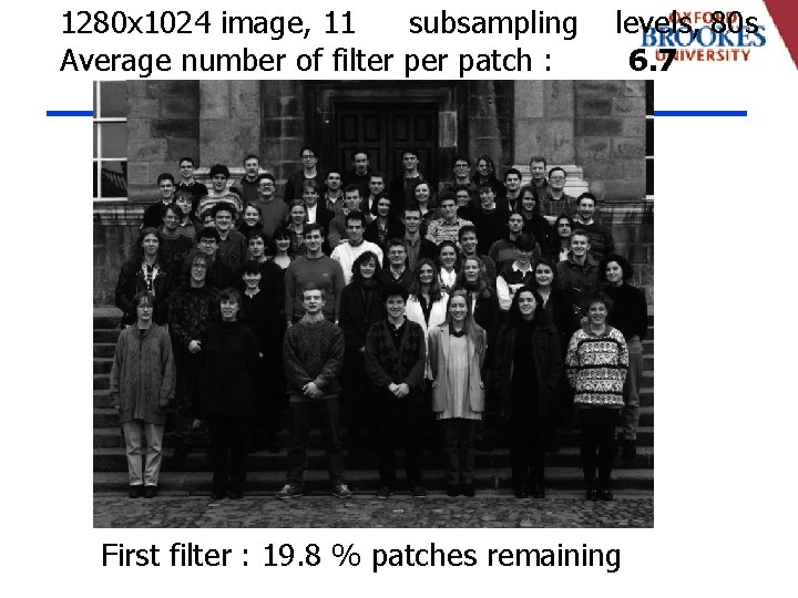
1280 x 1024 image, 11 subsampling Average number of filter patch : levels, 80 s 6. 7 First filter : 19. 8 % patches remaining

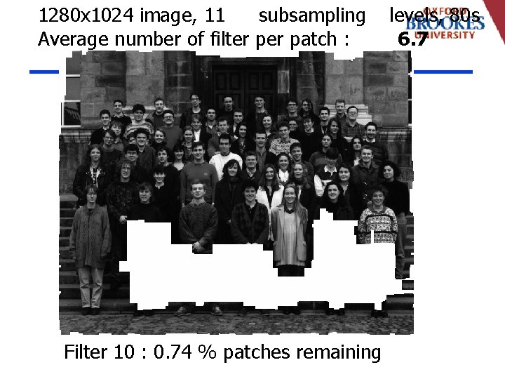
1280 x 1024 image, 11 subsampling Average number of filter patch : Filter 10 : 0. 74 % patches remaining levels, 80 s 6. 7

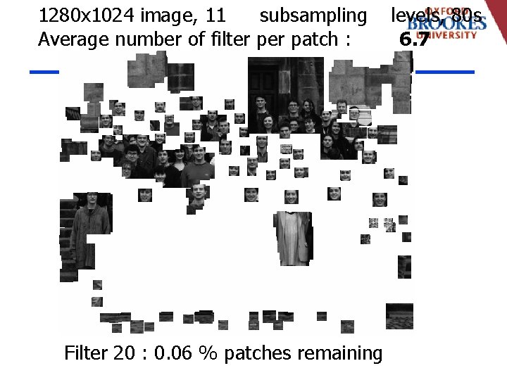
1280 x 1024 image, 11 subsampling Average number of filter patch : Filter 20 : 0. 06 % patches remaining levels, 80 s 6. 7

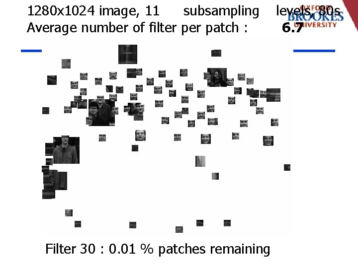
1280 x 1024 image, 11 subsampling Average number of filter patch : Filter 30 : 0. 01 % patches remaining levels, 80 s 6. 7

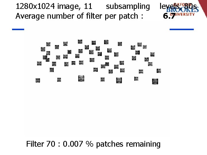
1280 x 1024 image, 11 subsampling Average number of filter patch : levels, 80 s 6. 7 Filter 70 : 0. 007 % patches remaining

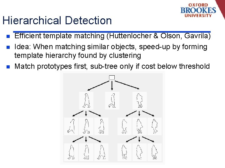
Hierarchical Detection n Efficient template matching (Huttenlocher & Olson, Gavrila) Idea: When matching similar objects, speed-up by forming template hierarchy found by clustering Match prototypes first, sub-tree only if cost below threshold

Trees n These search trees are the same as used for efficient nearest neighbour. n Add dynamic model and • Detection = Tracking = Recognition

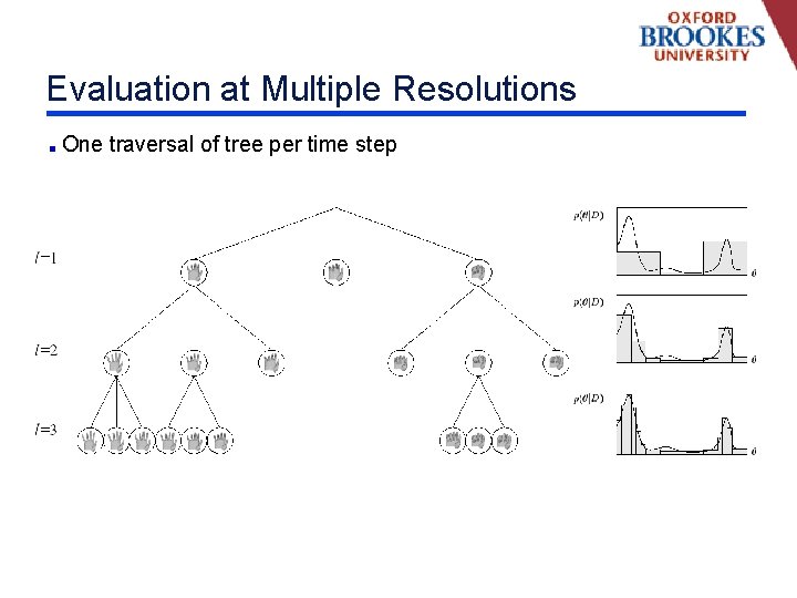
Evaluation at Multiple Resolutions One traversal of tree per time step

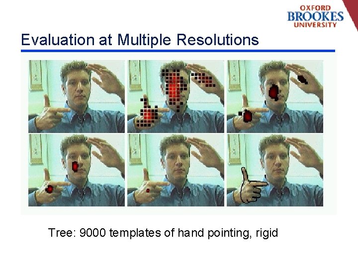
Evaluation at Multiple Resolutions Tree: 9000 templates of hand pointing, rigid

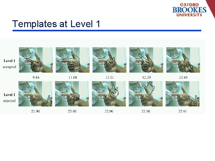
Templates at Level 1

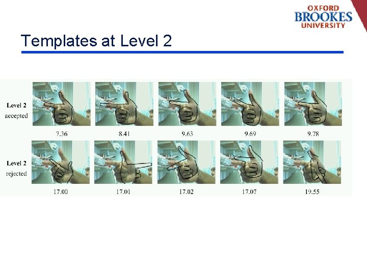
Templates at Level 2

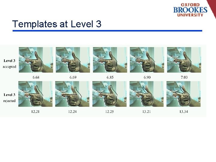
Templates at Level 3

Comparison with Particle Filters n This method is grid based, • No need to render the model on line • Like efficient search • Can always use this as a proposal process for a particle filter if need be.

Interpolation, MVRVM, ECCV 2006 Code available.

Energy being Optimized, link to graph cuts n Combination of • Edge term (quickly evaluated using chamfer) • Interior term (quickly evaluated using integral images) n Note that possible templates are a bit like cuts that we put down, one could think of this whole process as a constrained search for the best graph cut.

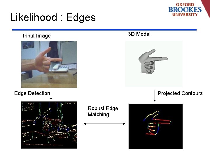
Likelihood : Edges 3 D Model Input Image Edge Detection Projected Contours Robust Edge Matching

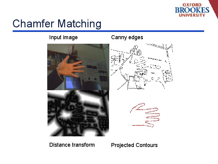
Chamfer Matching Input image Canny edges Distance transform Projected Contours

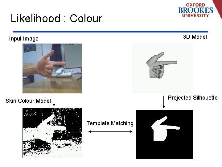
Likelihood : Colour 3 D Model Input Image Projected Silhouette Skin Colour Model Template Matching

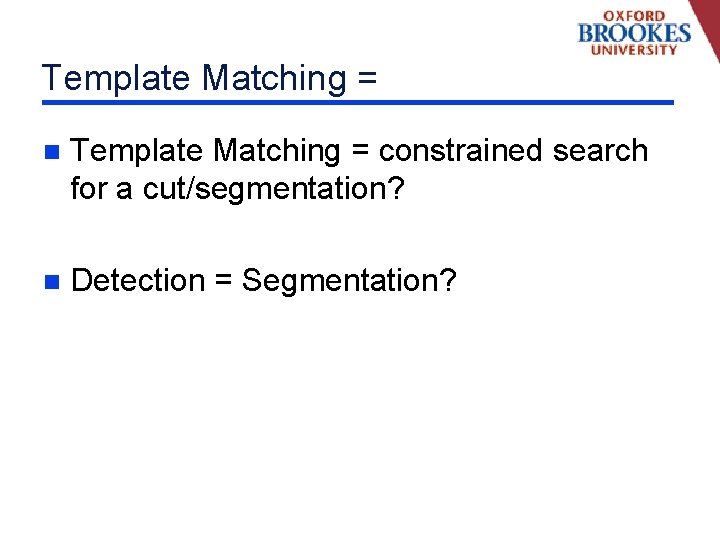
Template Matching = n Template Matching = constrained search for a cut/segmentation? n Detection = Segmentation?

Objective Aim to get a clean segmentation of a human… Image Segmentation Pose Estimate? ?

MRF for Interactive Image Segmentation, Boykov and Jolly [ICCV 2001] Energy. MRF = Unary likelihood Contrast Term Uniform Prior (Potts Model) Maximum-a-posteriori (MAP) solution x* = arg min E(x) x Data (D) Unary likelihood Pair-wise Terms MAP Solution

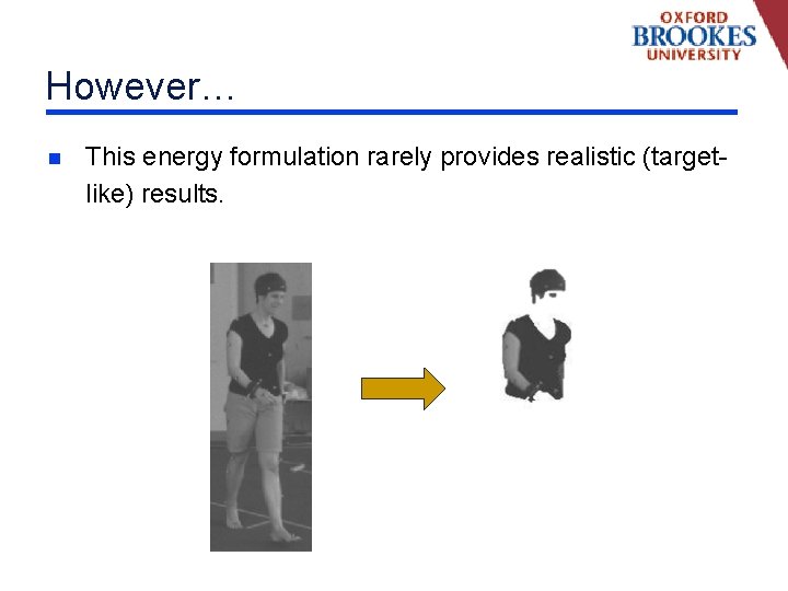
However… n This energy formulation rarely provides realistic (targetlike) results.

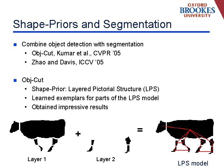
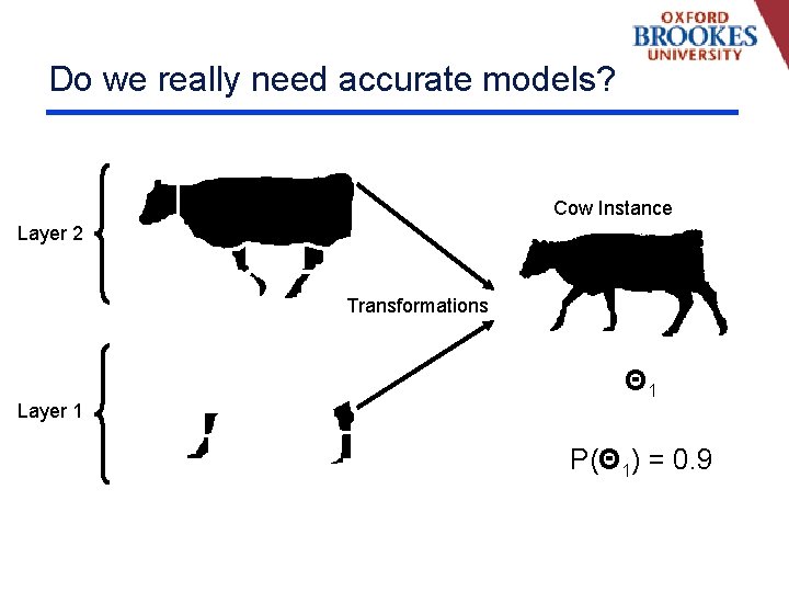
Shape-Priors and Segmentation n Combine object detection with segmentation • Obj-Cut, Kumar et al. , CVPR ’ 05 • Zhao and Davis, ICCV ’ 05 n Obj-Cut • Shape-Prior: Layered Pictorial Structure (LPS) • Learned exemplars for parts of the LPS model • Obtained impressive results = + Layer 1 Layer 2 LPS model

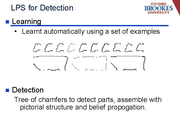
LPS for Detection n Learning • Learnt automatically using a set of examples n Detection Tree of chamfers to detect parts, assemble with pictorial structure and belief propogation.

Solve via Integer Programming n SDP formulation (Torr 2001, AI stats) n SOCP formulation (Kumar, Torr & Zisserman this conference) n LBP (Huttenlocher, many)

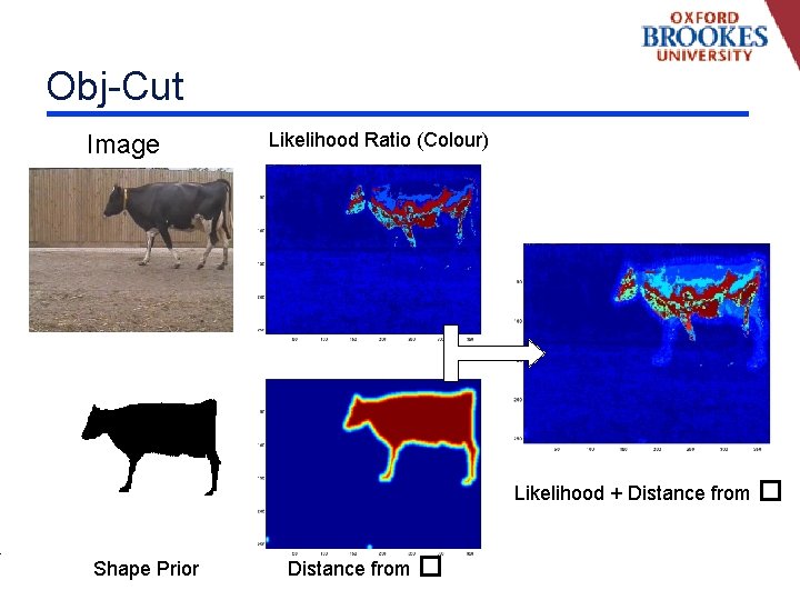
Obj-Cut Image Likelihood Ratio (Colour) Likelihood + Distance from � Shape Prior Distance from �

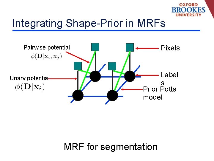
Integrating Shape-Prior in MRFs Pixels Pairwise potential Unary potential Label s Prior Potts model MRF for segmentation

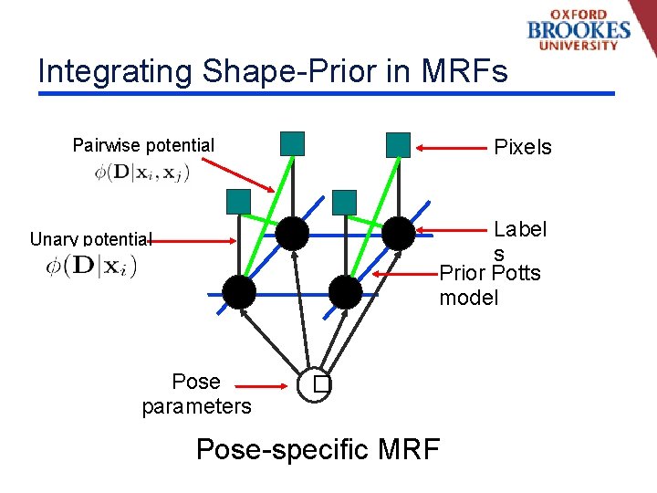
Integrating Shape-Prior in MRFs Pixels Pairwise potential Label s Prior Potts model Unary potential Pose parameters � Pose-specific MRF

Do we really need accurate models? Cow Instance Layer 2 Transformations Layer 1 Θ 1 P(Θ 1) = 0. 9

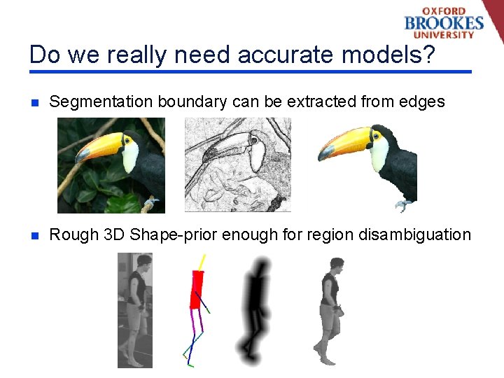
Do we really need accurate models? n Segmentation boundary can be extracted from edges n Rough 3 D Shape-prior enough for region disambiguation

Energy of the Pose-specific MRF Energy to be minimized Pairwise potential Unary term Potts model Shape prior But what should be the value of θ?

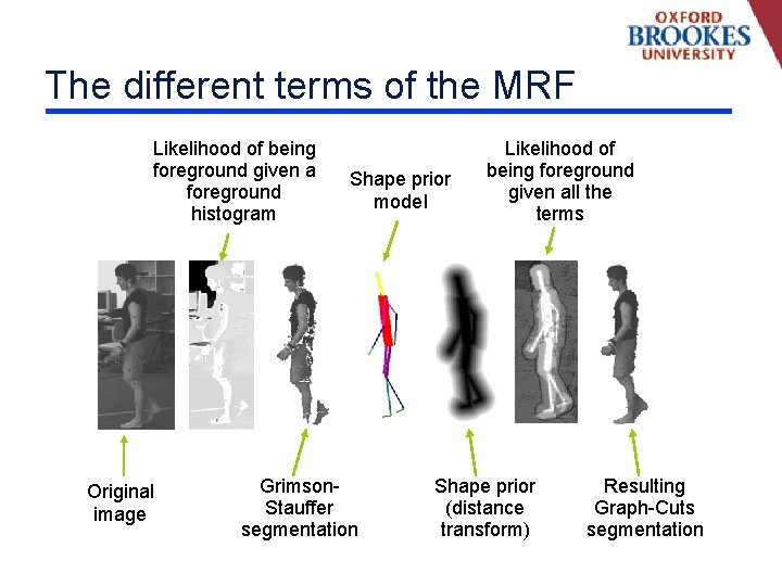
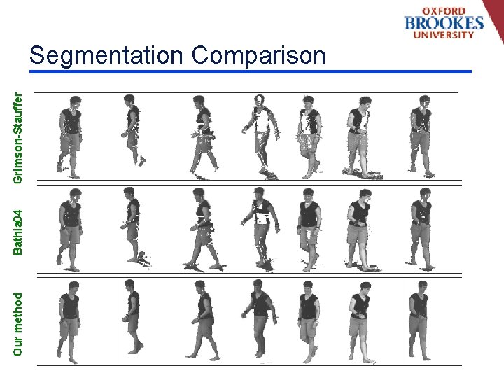
The different terms of the MRF Likelihood of being foreground given a foreground histogram Original image Shape prior model Grimson. Stauffer segmentation Likelihood of being foreground given all the terms Shape prior (distance transform) Resulting Graph-Cuts segmentation

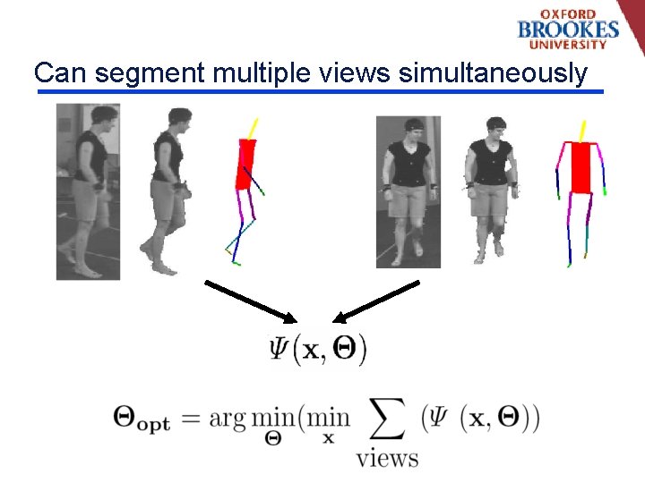
Can segment multiple views simultaneously

Solve via gradient descent n Comparable to level set methods n Could use other approaches (e. g. Objcut) n Need a graph cut per function evaluation

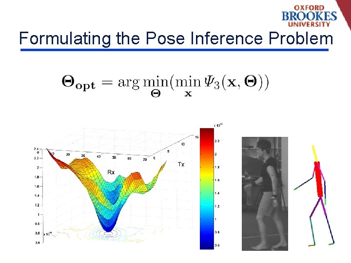
Formulating the Pose Inference Problem

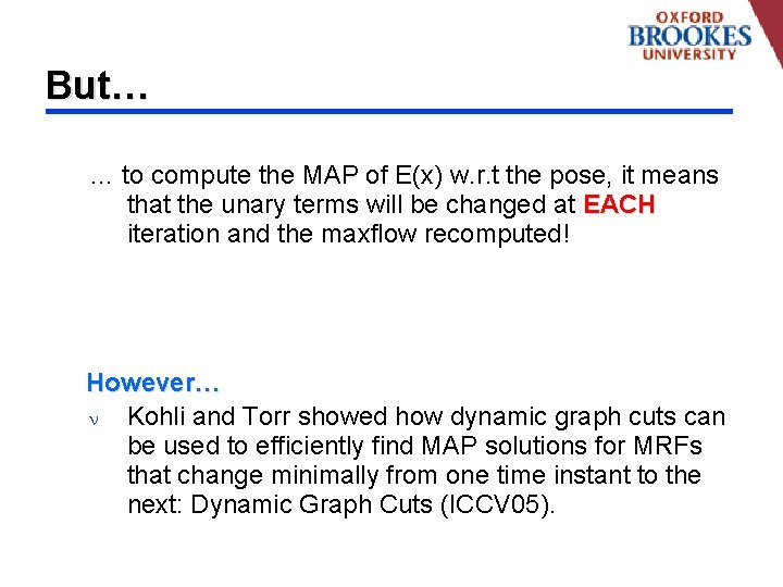
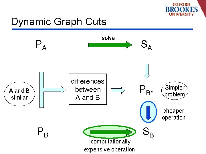
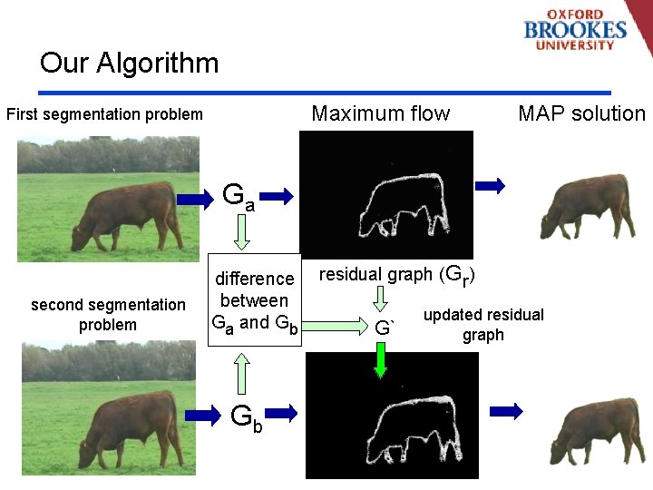
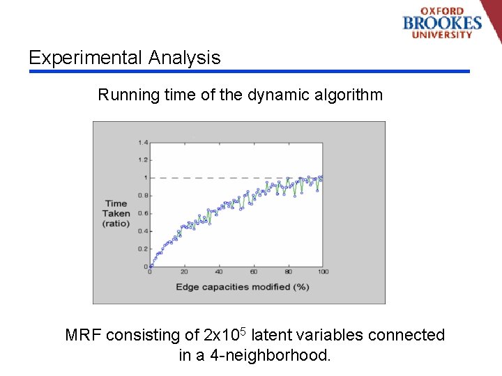
But… … to compute the MAP of E(x) w. r. t the pose, it means that the unary terms will be changed at EACH iteration and the maxflow recomputed! However… n Kohli and Torr showed how dynamic graph cuts can be used to efficiently find MAP solutions for MRFs that change minimally from one time instant to the next: Dynamic Graph Cuts (ICCV 05).

Dynamic Graph Cuts PA solve differences between A and B similar SA PB* Simpler problem cheaper operation PB computationally expensive operation SB

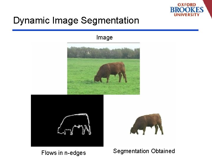
Dynamic Image Segmentation Image Flows in n-edges Segmentation Obtained

Our Algorithm Maximum flow First segmentation problem MAP solution Ga second segmentation problem difference between Ga and Gb Gb residual graph (Gr) G` updated residual graph

Dynamic Graph Cut vs Active Cuts n Our method flow recycling n AC cut recycling n Both methods: Tree recycling

Experimental Analysis Running time of the dynamic algorithm MRF consisting of 2 x 105 latent variables connected in a 4 -neighborhood.

Our method Bathia 04 Grimson-Stauffer Segmentation Comparison

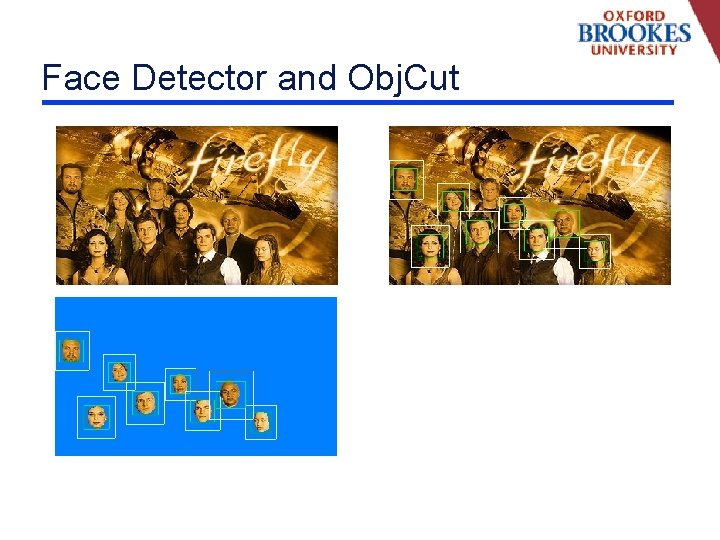
Face Detector and Obj. Cut

Segmentation

Segmentation

Conclusion n Combining pose inference and segmentation worth investigating. Tracking = Detection n Detection = Segmentation n Tracking = Segmentation. n Segmentation = SFM ? ? n