Simultaneous Optimization Ashish Goel University of Southern California

Simultaneous Optimization Ashish Goel University of Southern California Joint work with Deborah Estrin, UCLA (Concave Costs) Adam Meyerson, Stanford/CMU (Convex Costs, Concave Utilities) http: //cs. usc. edu/~agoel@cs. usc. edu

Algorithms/Theory of Computation at USC • • • Len Adleman Tim Chen Ashish Goel Ming-Deh Huang Mike Waterman Applications/Variations: – Arbib, Desbrun, Schaal, Sukhatme, Tavare… agoel@cs. usc. edu

My Long Term Research Agenda • Foundations of computer science (computation/interaction/information) – Combinatorial optimization – Approximation algorithms – Discrete Applied Probability • Find interesting connections – Operations research; queueing theory; stochastic processes; functional analysis; game theory • Find interesting application domains – Communication Networks – Self-Assembly agoel@cs. usc. edu

Simultaneous Optimization • Approximately minimize the cost of a system simultaneously for a large family of cost functions – Concave cost functions correspond to economies of scale – Convex cost functions measure congestion on machines, on agents, or in networks • Maximizing utility/profit without knowing the profit function – Allocated bandwidths to customers in a network – Concave profit functions correspond to the “law” of diminishing returns agoel@cs. usc. edu

Example of Concave Utilities: Revenue Maximization in Networks • Let x = hx 1, x 2, …, x. Ni denote the bandwidth allocated to N users in a communication network – These bandwidths must satisfy some linear capacity constraints, say Ax · C – Let U(x) denote the total revenue (or the utility) that the network operator can derive from the system • Goal: Maximize U(x), subject to Ax · C – x can be thought of as “wealth” in any resource allocation problem agoel@cs. usc. edu

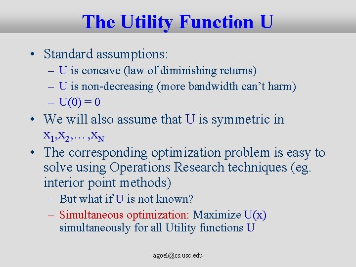
The Utility Function U • Standard assumptions: – U is concave (law of diminishing returns) – U is non-decreasing (more bandwidth can’t harm) – U(0) = 0 • We will also assume that U is symmetric in x 1, x 2, …, x. N • The corresponding optimization problem is easy to solve using Operations Research techniques (eg. interior point methods) – But what if U is not known? – Simultaneous optimization: Maximize U(x) simultaneously for all Utility functions U agoel@cs. usc. edu

Why simultaneous optimization? • Often, the utility function is poorly understood, eg. Customer satisfaction • Often, we might want to promote several different objectives, eg. Fairness • Let us focus on fairness. Should we – Maximize the average utility? – Be Max-min fair (steal from the rich)? – Maximize the average income of the bottom half of society? – Minimize the variance? – Do all of the above? agoel@cs. usc. edu

Fair Allocation Problem: Example • How to split a pie fairly? • But what if there are more constraints? • Alice and Eddy want only apple pie • Frank: allergic to apples • Cathy: equal portions of both pies • David: twice as much apple pie as lemon What is a “Fair” allocation? How do we find one? agoel@cs. usc. edu

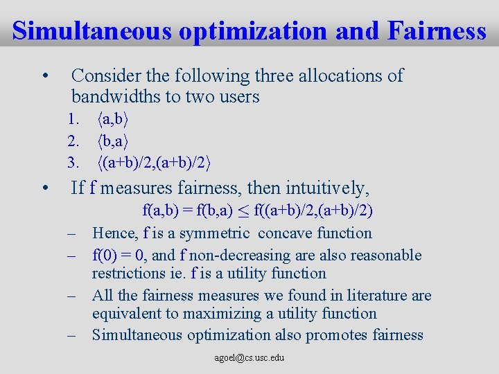
Simultaneous optimization and Fairness • Consider the following three allocations of bandwidths to two users 1. ha, bi 2. hb, ai 3. h(a+b)/2, (a+b)/2 i • If f measures fairness, then intuitively, – – f(a, b) = f(b, a) · f((a+b)/2, (a+b)/2) Hence, f is a symmetric concave function f(0) = 0, and f non-decreasing are also reasonable restrictions ie. f is a utility function All the fairness measures we found in literature are equivalent to maximizing a utility function Simultaneous optimization also promotes fairness agoel@cs. usc. edu

Can we do Simultaneous Optimization? • Of course not • But, perhaps we can do it “approximately”? – Aha!! Theoretical Computer Science! • More modest goal: – Find x subject to Ax · C, such that for any utility function U, U(x) is a good approximation to the maximum achievable value of U agoel@cs. usc. edu

Approximate Majorization • Given an allocation y of bandwidths to users, let Pi(y) denote the sum of the i smallest components of y – Let Pi* denote the largest possible value of Pi(y) • Definition: x is said to be a-majorized if Pi(x) ¸ Pi*/a for all 1· i· N – Variant of the notion of majorization – Interpretation: the K poorest individuals in the allocation x are collectively at least 1/a times as rich as the K poorest individuals in any other feasible allocation agoel@cs. usc. edu

Why Approximate Majorization? • Theorem 1: An allocation x is a-majorized if and only if U(x) is an a-approximation to the maximum possible value of U for all utility functions U – ie. a-majorization results in approximate simultaneous optimization – Proof invokes a classic theorem of Hardy, Littlewood, and Polya from the 1920 s agoel@cs. usc. edu

Existence • Theorem 2: For the bandwidth allocation problem in networks, there exists an O(log N)-majorized solution – ie. Can simultaneously approximate all utility functions up to a factor O(log N) • Results extend to arbitrary linear (even convex) programs, and not just the bandwidth allocation problem agoel@cs. usc. edu

Tractability • Theorem 3: Given arbitrary linear constraints, we can find (in polynomial time) the smallest a such that an amajorized solution exists – Can also find the corresponding a-majorized solution • This completes the study of approximate simultaneous optimization for linear programs [Goel, Meyerson; Unpublished] [Bhargava, Goel, Meyerson; short abstract in Sigmetrics ’ 01] agoel@cs. usc. edu

Examples of Utility Functions • • Min Pi(x) Sum/Average åi f(xi) where f is a uni-variate utility function – Eg. Entropy, åilog (1+xi) etc. • Variance is also symmetric convex – Can also approximately minimize the variance Can simultaneously approximate capitalism, communism, and many other “ism”s. agoel@cs. usc. edu

Open Problem Distributed Algorithms? ? agoel@cs. usc. edu

Example of Concave Costs: Data Aggregation in Sensor Networks • There is a single sink and multiple sources of information – Need to construct an aggregation tree – Data flows from the sources to the sink along the tree – When two data streams collide, they aggregate • Let f(k) denote the size of k merged streams – Assume f(0) = 0, f is concave, f is non-decreasing • Concavity corresponds to concavity of entropy/information – Canonical Aggregation Functions • The amount of aggregation might depend on nature of information – f is not known in advance agoel@cs. usc. edu

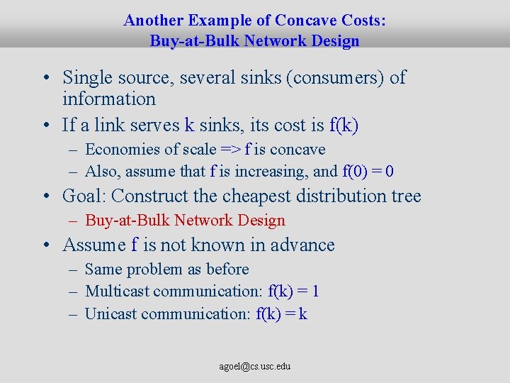
Another Example of Concave Costs: Buy-at-Bulk Network Design • Single source, several sinks (consumers) of information • If a link serves k sinks, its cost is f(k) – Economies of scale => f is concave – Also, assume that f is increasing, and f(0) = 0 • Goal: Construct the cheapest distribution tree – Buy-at-Bulk Network Design • Assume f is not known in advance – Same problem as before – Multicast communication: f(k) = 1 – Unicast communication: f(k) = k agoel@cs. usc. edu

A Simple Algorithmic Trick Jensen’s Inequality • • E[f(X)] · f(E[X]) for any concave function f Hence, given a fractional/multipath solution, randomized rounding can only help 2 Prob. ½ 1 source 0. 5 sink Prob. ¼ 2 agoel@cs. usc. edu

Notation • Given graph G=(V, E) and – – Cost function c : E! <+ on edges Sink t Set S of K sources Cost of supporting j users on edge e is c(e)f(j), where f is an unknown canonical aggregation function • Given an aggregation tree T, CT(f) = Cost of tree T for function f – C*(f) = min. T{CT(f)} – RT(f) = CT(f)/ C*(f) agoel@cs. usc. edu

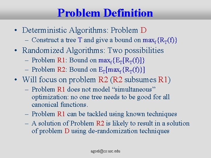
Problem Definition • Deterministic Algorithms: Problem D – Construct a tree T and give a bound on maxf{RT(f)} • Randomized Algorithms: Two possibilities – Problem R 1: Bound on maxf{ET[RT(f)]} – Problem R 2: Bound on ET[maxf{RT(f)}] • Will focus on problem R 2 (R 2 subsumes R 1) – Problem R 1 does not model “simultaneous” optimization: no one tree needs to be good for all canonical functions. – Problem R 1 can be tackled using known techniques – A solution of Problem R 2 is likely to result in a solution of problem D using de-randomization techniques agoel@cs. usc. edu

Previous Work • Problem is NP-Hard even when f is known – Randomized O(log K) approximation for problem R 1 using Bartal’s tree embeddings [Bartal ’ 98; Awerbuch and Azar ’ 97] – Improved to a constant factor [Guha, Meyerson, Munagala ‘ 01] • O(log K) approximation when f is known, but can be different for different links [Meyerson, Munagala, Plotkin ’ 00] agoel@cs. usc. edu

Background: Bartal’s Result • Randomized algorithm which takes an arbitrary metric space (V, d. V) as input and constructs a tree metric (V, d. T) such that d. V(u, v) · d. T(u, v), and E[d. T(u, v)] · a d. V(u, v), where a = O(log n) • Results in an O(log K) guarantee for problem R 1 – No obvious way to extend to problem R 2 – Quite complicated agoel@cs. usc. edu

Our Results • Simple Algorithm – Gives a bound of 1 + log K for problem R 2 – Intreresting rules of thumb • Can be de-randomized using pessimistic estimators and the O(1) approximation algorithm for known f – Quite technical; details omitted agoel@cs. usc. edu

Our Algorithm: Hierarchical Matching 1. Find the minimum cost matching between sources • • The “Matching” Step cost is measured in terms of shortest path distance 2. For each matched pair, pick one at random and discard it • • The “Random Selection” Step Pretend that the demand from the discarded node is moved to the remaining node 3. If two or more sources remain, go back to step 1 4. At the end, take a union of all the matchings and also connect the single remaining source to the sink agoel@cs. usc. edu

Example Demands are all 1 Sink agoel@cs. usc. edu

Example Demands are all 1 Matching 1 agoel@cs. usc. edu

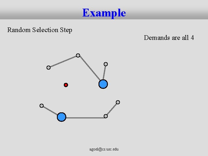
Example Random Selection Step Demands are all 2 agoel@cs. usc. edu

Example Demands are all 2 Matching 2 agoel@cs. usc. edu

Example Random Selection Step Demands are all 4 agoel@cs. usc. edu

Example Demands are all 4 Matching 3 agoel@cs. usc. edu

Example Random Selection Step Demands are all 8 agoel@cs. usc. edu

Example: The Final Solution 1 2 1 8 4 1 2 1 agoel@cs. usc. edu • Mi = Total cost of edges in i-th matching • CT(f) = åi Mi f(2 i-1)

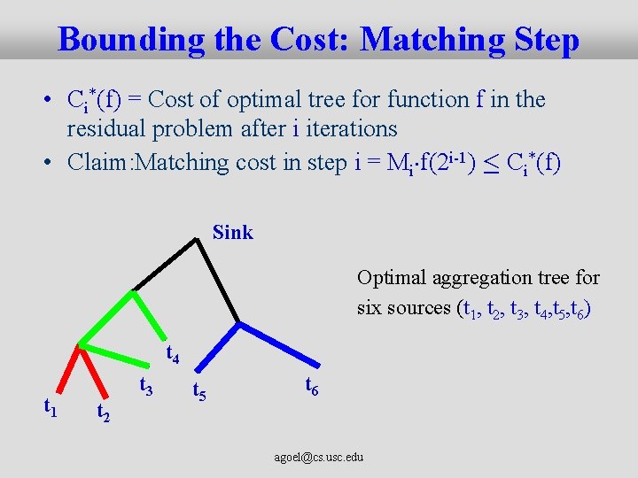
Bounding the Cost: Matching Step • Ci*(f) = Cost of optimal tree for function f in the residual problem after i iterations • Claim: Matching cost in step i = Mi¢f(2 i-1) · Ci*(f) Sink Optimal aggregation tree for six sources (t 1, t 2, t 3, t 4, t 5, t 6) t 4 t 1 t 2 t 3 t 5 t 6 agoel@cs. usc. edu

Bounding the Cost: Random Selection • Consider any edge e in the optimum aggregation tree for function f – Let k(e) be the number of sinks which use e • Focus on the “Random selection” step for one matched pair (u, v) – k’(e) = total demand routed on edge e after this step – For each of u and v, the demand is doubled with probability ½ and becomes 0 otherwise => E[k’(e)] = k(e) • By Jensen’s inequality: E[f(k’(e)] · f[E[k’(e)] = f(k(e)) agoel@cs. usc. edu

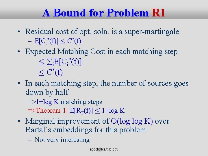
A Bound for Problem R 1 • Residual cost of opt. soln. is a super-martingale – E[Ci*(f)] · C*(f) • Expected Matching Cost in each matching step · åi. E[Ci*(f)] · C*(f) • In each matching step, the number of sources goes down by half =>1+log K matching steps =>Theorem 1: E[RT(f)] · 1+log K • Marginal improvement of O(log K) over Bartal’s embeddings for this problem – Not very interesting agoel@cs. usc. edu

Bound for Problem R 2 • Atomic aggregation functions – Ai(x) = min{x, 2 i} Ai(x) 2 i x • Ai is a canonical aggregation function • Main Idea: Suffices to study the performance of our algorithm just for the atomic functions Details complicated; Omitted agoel@cs. usc. edu

Open Algorithmic Problems • Multicommodity version (many source-sink pairs) – Preliminary Progress: Can obtain O(log n log K log n) guarantee using Bartal’s embeddings combined with our analysis • Lower Bounds? – Conjecture: W(log K) • Handle arbitrary demands at sinks – Our algorithm yields 1 + log K + log D guarantee for problem R 2 where D is the maximum demand agoel@cs. usc. edu

Open Modeling Problems Realistic models of more general aggregation functions • Information cancellation – One node senses a pest infestation and sends an alarm. – Another node senses high pesticide levels in the atmosphere, and sends another alarm. – An intermediate node might receive both pieces of information and suppress both alarms. • Amount of aggregation may depend on the set of nodes being aggregated rather than just the number – Concave function f(Se) as opposed to f(ke) – Bartal’s algorithm still gives an O(log K) guarantee for problem R 1 agoel@cs. usc. edu

Moral • Why settle for one cost function when you can approximate them all? – Argument against approximate modeling of aggregation functions • Particularly useful for poorly understood or inherently multi-criteria problems – “Information independent” aggregation agoel@cs. usc. edu