Simultaneous Buffer Insertion and Wire Sizing Considering Systematic

Simultaneous Buffer Insertion and Wire Sizing Considering Systematic CMP Variation and Random Leff Variation Lei He 1, Andrew Kahng 2, King Ho Tam 1, Jinjun Xiong 1 1 Univ. of California, Los Angeles 2 Blaze DFM, Inc. & Univ. of California, San Diego Sponsors: 1 NSF CAREER, SRC, UC MICRO sponsored by Analog Devices, Fujitsu Lab. , Intel and LSI Logic, IBM Faculty Partner Award; 2 MARCO Gigascale System Research Center, NSF.

Existing Work on Variation. Aware Buffer Insertion l Buffer insertion for length variation [Khandelwal-ICCAD] l l Variation sources from difference between estimated and actual wire length Buffer insertion for process variation [Xiong. DATE] l l Random Leff and interconnect width variations Brute-force numerical manipulation of joint probability density functions (JPDFs), not efficient

Buffer Insertion and Wire Sizing (SBW) with Process Variations l Variations models l l l Leff – random variation l In reality, 50% systematic and 50% random Interconnect RC – systematic variation due to Chemical Mechanical Planarization (CMP) l Random component of global interconnect variation on performance is insignificant in general Efficient variation-aware algorithms l l Table-based capacitance and fill insertion under CMP Efficient pruning to deal with random variation

Outline l SBW and fill insertion (SBWF) under CMP variation l l l Modeling RC variation CMP-aware SBW and fill insertion algorithm Experiment: CMP-aware vs CMP-oblivious Extension to Leff variation Conclusion

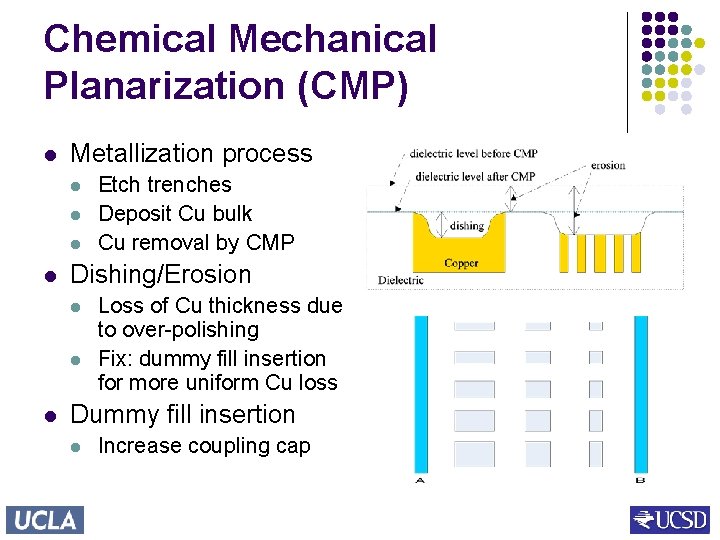
Chemical Mechanical Planarization (CMP) l Metallization process l l Dishing/Erosion l l l Etch trenches Deposit Cu bulk Cu removal by CMP Loss of Cu thickness due to over-polishing Fix: dummy fill insertion for more uniform Cu loss Dummy fill insertion l Increase coupling cap

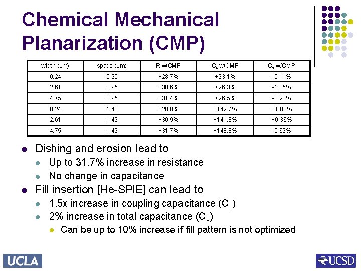
Chemical Mechanical Planarization (CMP) l space (μm) R w/CMP Cc w/CMP Cs w/CMP 0. 24 0. 95 +28. 7% +33. 1% -0. 11% 2. 61 0. 95 +30. 6% +26. 3% -1. 35% 4. 75 0. 95 +31. 4% +26. 5% -0. 23% 0. 24 1. 43 +28. 8% +142. 7% +1. 88% 2. 61 1. 43 +30. 9% +141. 8% +0. 36% 4. 75 1. 43 +31. 7% +148. 8% -0. 69% Dishing and erosion lead to l l l width (μm) Up to 31. 7% increase in resistance No change in capacitance Fill insertion [He-SPIE] can lead to l l 1. 5 x increase in coupling capacitance (Cc) 2% increase in total capacitance (Cs) l Can be up to 10% increase if fill pattern is not optimized

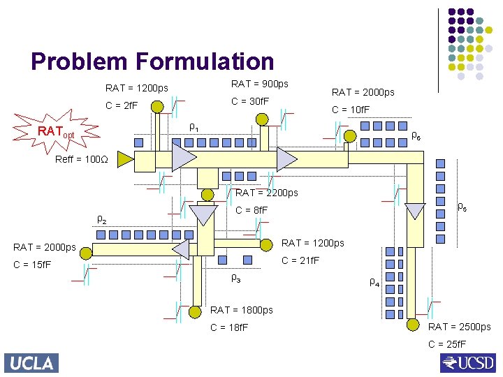
Problem Formulation RAT = 1200 ps RAT = 900 ps C = 2 f. F C = 30 f. F RAT = 2000 ps C = 10 f. F ρ1 RATopt ρ6 Reff = 100Ω RAT = 2200 ps ρ2 ρ5 C = 8 f. F RAT = 2000 ps RAT = 1200 ps C = 15 f. F C = 21 f. F ρ3 ρ4 RAT = 1800 ps C = 18 f. F RAT = 2500 ps C = 25 f. F

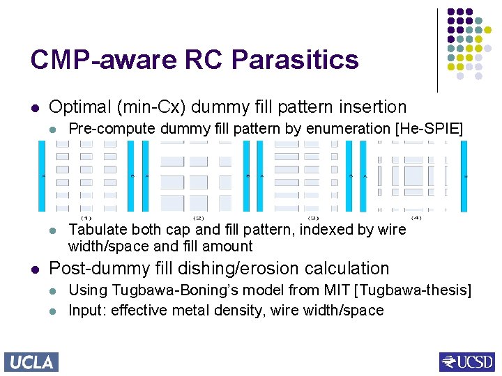
CMP-aware RC Parasitics l l Optimal (min-Cx) dummy fill pattern insertion l Pre-compute dummy fill pattern by enumeration [He-SPIE] l Tabulate both cap and fill pattern, indexed by wire width/space and fill amount Post-dummy fill dishing/erosion calculation l l Using Tugbawa-Boning’s model from MIT [Tugbawa-thesis] Input: effective metal density, wire width/space

SBWF Algorithm l Extended dynamic programming [van Ginneken-ISCS] l CMP model is deterministic l l l Amount of variation calculated from metal features Use CMP-aware RC Prune sub-optimal/invalid partial solutions l l Inferior: Cinf > Cn & ATint < ATn Rise-time violation: Dsubtree > Dbound

Experiment l Experimental settings l l l ITRS 65 nm (interconnect) & BSIM 4 (device) RAT at sinks = 0, Tr < 100 ps SBW + Fill l Solving SBW using CMP-oblivious RC, i. e. no dishing/erosion/fill insertion l l l Risetime constraint set to 83 ps during optimization to get solution that meets the Tr < 100 ps constraint Solution to be verified after under CMP-aware RC SBWF l Simultaneous buffering, wire sizing and fill insertion

Experiment: SBW + Fill vs SBWF r 1 – r 5: benchmarks from [Tsay-TCAD] l SBW + Fill l SBWF net # sinks Src AT (ps) Power (p. J) Runtime (s) r 1 267 -2437 266 67 -2427 (0. 4%) 250 (-6. 2%) 86 r 2 598 -3080 531 173 -3044 (1. 2%) 486 (-8. 5%) 193 r 3 862 -3684 662 207 -3636 (1. 3%) 613 (-7. 4%) 257 r 4 1903 -5372 1358 389 -5319 (1. 0%) 1243 (-8. 5%) 459 r 5 3101 -6005 2025 512 -5960 (0. 7%) 1865 (-7. 9%) 727 SBWF improves over SBW + Fill design 1. 2. by 1. 0% arrival time on average by 5. 7% power per switch

Outline l SBW and fill insertion (SBWF) under CMP variation l l l Modeling RC variation CMP-aware SBW and fill insertion algorithm Experiment: CMP-aware vs CMP-oblivious Extension to Leff variation Conclusion

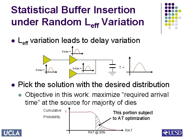
Statistical Buffer Insertion under Random Leff Variation l Leff variation leads to delay variation Delay = l T= Delay = Pick the solution with the desired distribution l Objective in this work: maximize “required arrival time” at the source for majority of dies Cumulative 1 This portion subject to AT optimization Probability RAT @ 90% RAT

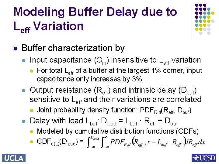
Modeling Buffer Delay due to Leff Variation l Buffer characterization by l Input capacitance (Cin) insensitive to Leff variation l l Output resistance (Reff) and intrinsic delay (Dbuf) sensitive to Leff and their variations are correlated l l For total Leff of a buffer at the largest 1% corner, input capacitance only increases by 3% Joint probability density function: PDFR, d(Reff, Dbuf) Delay with load Lbuf: Dload = Lbuf · Reff + Dbuf l l Modeled by cumulative distribution functions (CDFs) CDFd(L)(Dload) =

Challenges in Statistical Buffer Insertion Problem l Efficient manipulation of statistical calculation l l l Arrival time as a random variable for optimization l Captured by CDF l Calculation is slow by brute-force manipulation Our approach: piece-wise linear (PWL) modeling Pruning rules to remove sub-optimal options l l Deterministic l AT 1 > AT 2 and L 1 < L 2 – establishes total order Probabilistic l P(AT 1 > AT 2 Λ L 1 < L 2) – only forms partial order § eg. P(AT 1 > AT 2) = 0. 6: sol 1 >> 2, but with a low probability

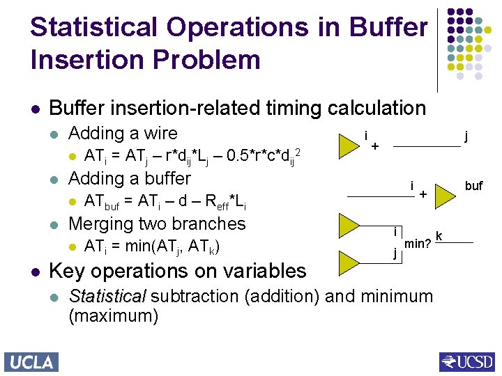
Statistical Operations in Buffer Insertion Problem l Buffer insertion-related timing calculation l Adding a wire l l ATi = min(ATj, ATk) Key operations on variables l + i ATbuf = ATi – d – Reff*Li Merging two branches l l j Adding a buffer l l ATi = ATj – r*dij*Lj – 0. 5*r*c*dij 2 i i j buf + min? Statistical subtraction (addition) and minimum (maximum) k

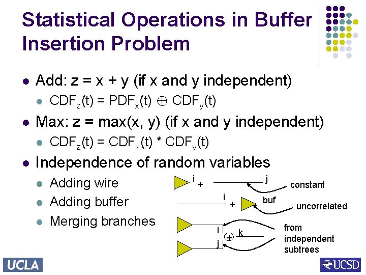
Statistical Operations in Buffer Insertion Problem l Add: z = x + y (if x and y independent) l l Max: z = max(x, y) (if x and y independent) l l CDFz(t) = PDFx(t) ⊕ CDFy(t) CDFz(t) = CDFx(t) * CDFy(t) Independence of random variables l l l Adding wire Adding buffer Merging branches i j + i k + j buf constant uncorrelated from independent subtrees

Modeling Cumulative Distribution Functions (CDFs) l CDF: PWL curve [Devgan-ICCAD] l Statistical addition (convolution) and maximum (multiplication) has closed-form solutions under PWL modeling l l l FAST!! Sampling at pre-set percentile points on the y-axis is performed after operations to keep PWL form PDF: Piecewise constant (PWC) curve l Obtained by differentiating the PWL of CDF

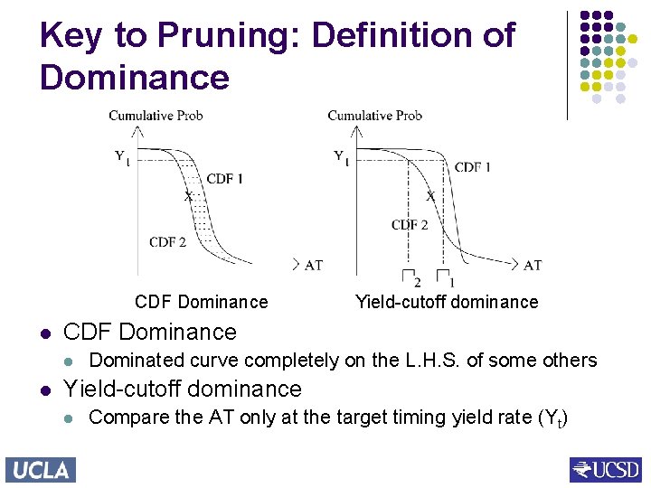
Key to Pruning: Definition of Dominance CDF Dominance l l Yield-cutoff dominance Dominated curve completely on the L. H. S. of some others Yield-cutoff dominance l Compare the AT only at the target timing yield rate (Yt)

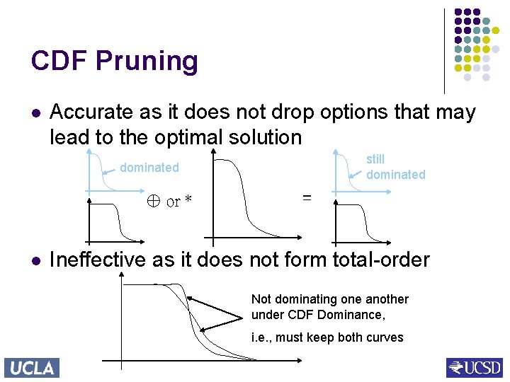
CDF Pruning l Accurate as it does not drop options that may lead to the optimal solution still dominated ⊕ or * l = Ineffective as it does not form total-order Not dominating one another under CDF Dominance, i. e. , must keep both curves

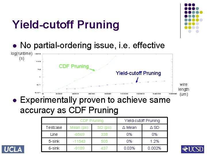
Yield-cutoff Pruning l No partial-ordering issue, i. e. effective log(runtime) (s) CDF Pruning Yield-cutoff Pruning l Experimentally proven to achieve same accuracy as CDF Pruning Yield-cutoff Pruning Testcase Mean (ps) SD (ps) Δ Mean Δ SD Line -6569 338 0% 0% 5 -sink -11543 505 0% 1. 2% 6 -sink -9189 437 0. 03% 0. 002% wire length (um)

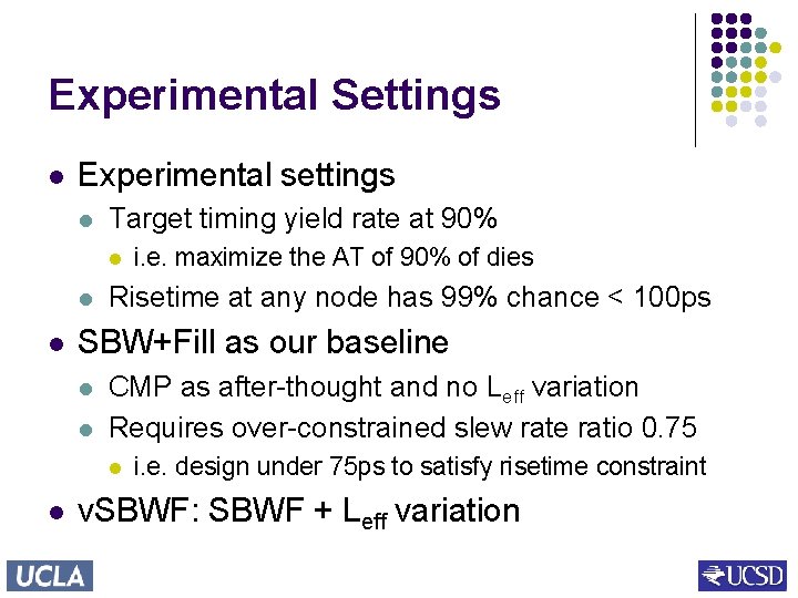
Experimental Settings l Experimental settings l Target timing yield rate at 90% l l l Risetime at any node has 99% chance < 100 ps SBW+Fill as our baseline l l CMP as after-thought and no Leff variation Requires over-constrained slew rate ratio 0. 75 l l i. e. maximize the AT of 90% of dies i. e. design under 75 ps to satisfy risetime constraint v. SBWF: SBWF + Leff variation

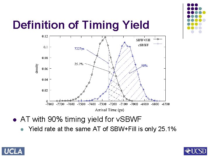
Definition of Timing Yield l AT with 90% timing yield for v. SBWF l Yield rate at the same AT of SBW+Fill is only 25. 1%

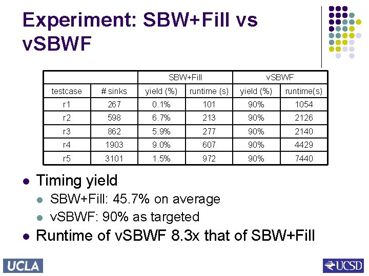
Experiment: SBW+Fill vs v. SBWF SBW+Fill l testcase # sinks yield (%) runtime (s) yield (%) runtime(s) r 1 267 0. 1% 101 90% 1054 r 2 598 6. 7% 213 90% 2126 r 3 862 5. 9% 277 90% 2140 r 4 1903 9. 0% 607 90% 4429 r 5 3101 1. 5% 972 90% 7440 Timing yield l l l v. SBWF SBW+Fill: 45. 7% on average v. SBWF: 90% as targeted Runtime of v. SBWF 8. 3 x that of SBW+Fill

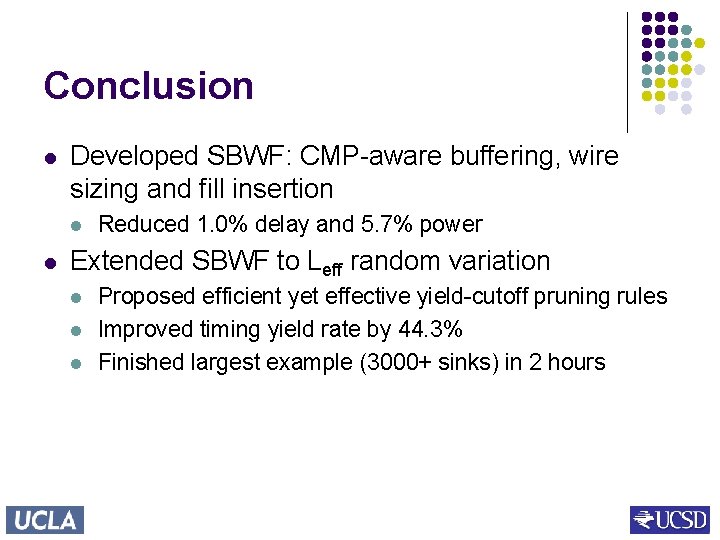
Conclusion l Developed SBWF: CMP-aware buffering, wire sizing and fill insertion l l Reduced 1. 0% delay and 5. 7% power Extended SBWF to Leff random variation l l l Proposed efficient yet effective yield-cutoff pruning rules Improved timing yield rate by 44. 3% Finished largest example (3000+ sinks) in 2 hours