Simulation Given a random variable X with CDF

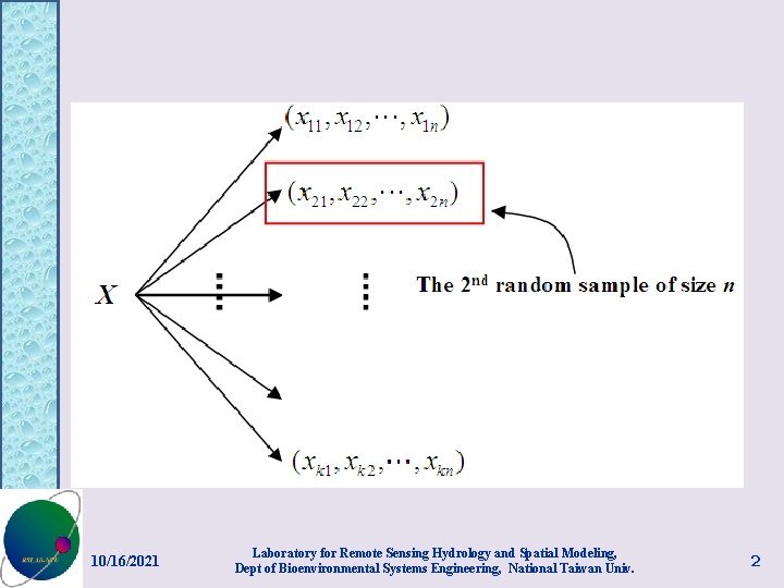
Simulation • Given a random variable X with CDF FX(x), there are situations that we want to obtain a set of n random numbers (i. e. , a random sample of size n) from FX(. ). • The advances in computer technology have made it possible to generate such random numbers using computers. The work of this nature is termed “simulation”, or more precisely “stochastic simulation”. 10/16/2021 Laboratory for Remote Sensing Hydrology and Spatial Modeling, Dept of Bioenvironmental Systems Engineering, National Taiwan Univ. 1

10/16/2021 Laboratory for Remote Sensing Hydrology and Spatial Modeling, Dept of Bioenvironmental Systems Engineering, National Taiwan Univ. 2

Pseudo-random number generation • Pseudorandom number generation (PRNG) is the technique of generating a sequence of numbers that appears to be a random sample of random variables uniformly distributed over (0, 1). 10/16/2021 Laboratory for Remote Sensing Hydrology and Spatial Modeling, Dept of Bioenvironmental Systems Engineering, National Taiwan Univ. 3

• A commonly applied approach of PRNG starts with an initial seed and the following recursive algorithm (Ross, 2002) modulo m where a and m are given positive integers, and the above equation means that is divided by m and the remainder is taken as the value of. 10/16/2021 Laboratory for Remote Sensing Hydrology and Spatial Modeling, Dept of Bioenvironmental Systems Engineering, National Taiwan Univ. 4

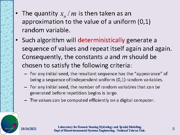
• The quantity is then taken as an approximation to the value of a uniform (0, 1) random variable. • Such algorithm will deterministically generate a sequence of values and repeat itself again and again. Consequently, the constants a and m should be chosen to satisfy the following criteria: – For any initial seed, the resultant sequence has the “appearance” of being a sequence of independent uniform (0, 1) random variables. – For any initial seed, the number of random variables that can be generated before repetition begins is large. – The values can be computed efficiently on a digital computer. 10/16/2021 Laboratory for Remote Sensing Hydrology and Spatial Modeling, Dept of Bioenvironmental Systems Engineering, National Taiwan Univ. 5

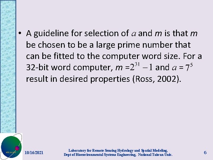
• A guideline for selection of a and m is that m be chosen to be a large prime number that can be fitted to the computer word size. For a 32 -bit word computer, m = and a = result in desired properties (Ross, 2002). 10/16/2021 Laboratory for Remote Sensing Hydrology and Spatial Modeling, Dept of Bioenvironmental Systems Engineering, National Taiwan Univ. 6

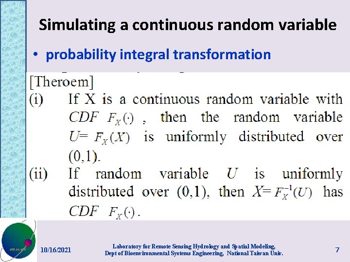
Simulating a continuous random variable • probability integral transformation 10/16/2021 Laboratory for Remote Sensing Hydrology and Spatial Modeling, Dept of Bioenvironmental Systems Engineering, National Taiwan Univ. 7

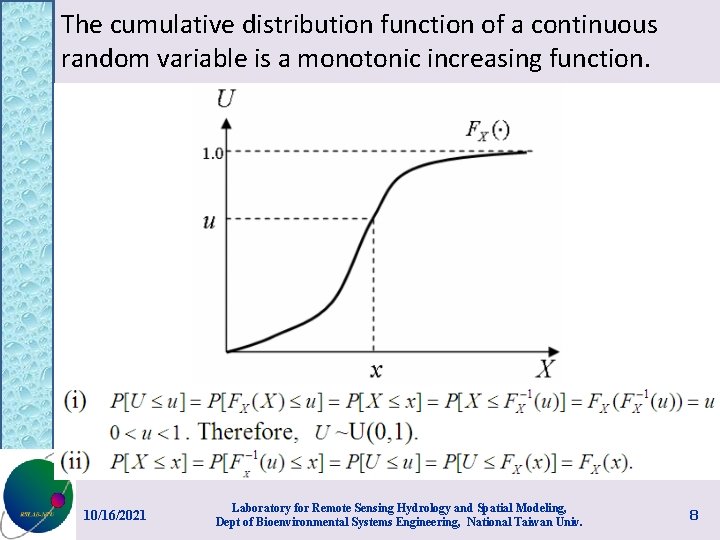
The cumulative distribution function of a continuous random variable is a monotonic increasing function. 10/16/2021 Laboratory for Remote Sensing Hydrology and Spatial Modeling, Dept of Bioenvironmental Systems Engineering, National Taiwan Univ. 8

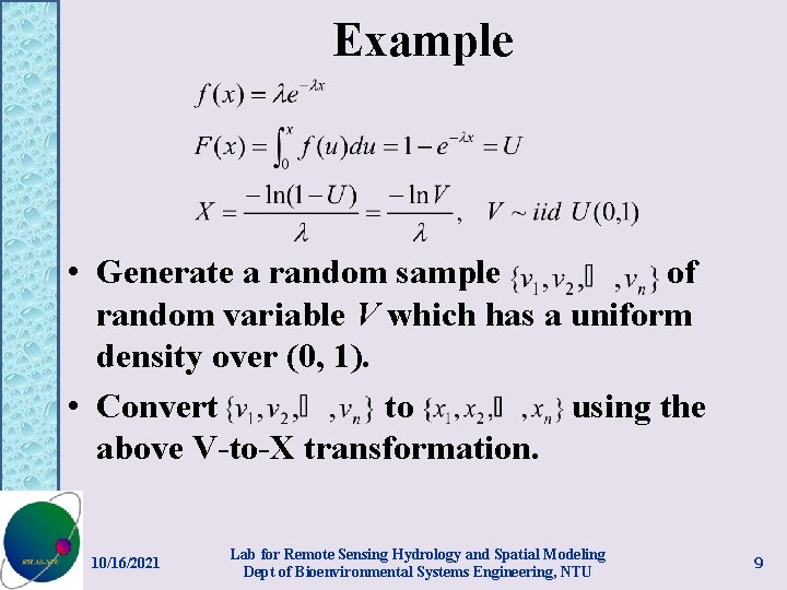
Example • Generate a random sample of random variable V which has a uniform density over (0, 1). • Convert to using the above V-to-X transformation. 10/16/2021 Lab for Remote Sensing Hydrology and Spatial Modeling Dept of Bioenvironmental Systems Engineering, NTU 9

10/16/2021 Lab for Remote Sensing Hydrology and Spatial Modeling Dept of Bioenvironmental Systems Engineering, NTU 10

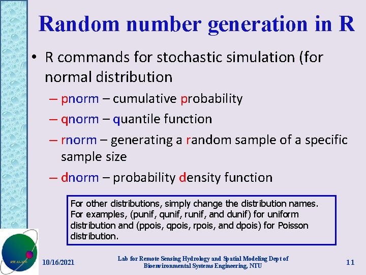
Random number generation in R • R commands for stochastic simulation (for normal distribution – pnorm – cumulative probability – qnorm – quantile function – rnorm – generating a random sample of a specific sample size – dnorm – probability density function For other distributions, simply change the distribution names. For examples, (punif, qunif, runif, and dunif) for uniform distribution and (ppois, qpois, rpois, and dpois) for Poisson distribution. 10/16/2021 Lab for Remote Sensing Hydrology and Spatial Modeling Dept of Bioenvironmental Systems Engineering, NTU 11

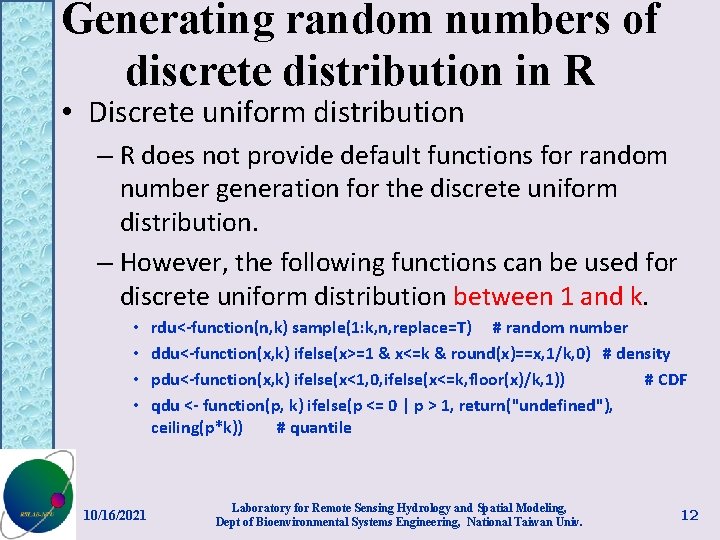
Generating random numbers of discrete distribution in R • Discrete uniform distribution – R does not provide default functions for random number generation for the discrete uniform distribution. – However, the following functions can be used for discrete uniform distribution between 1 and k. • • 10/16/2021 rdu<-function(n, k) sample(1: k, n, replace=T) # random number ddu<-function(x, k) ifelse(x>=1 & x<=k & round(x)==x, 1/k, 0) # density pdu<-function(x, k) ifelse(x<1, 0, ifelse(x<=k, floor(x)/k, 1)) # CDF qdu <- function(p, k) ifelse(p <= 0 | p > 1, return("undefined"), ceiling(p*k)) # quantile Laboratory for Remote Sensing Hydrology and Spatial Modeling, Dept of Bioenvironmental Systems Engineering, National Taiwan Univ. 12

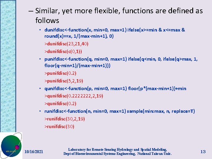
– Similar, yet more flexible, functions are defined as follows • dunifdisc<-function(x, min=0, max=1) ifelse(x>=min & x<=max & round(x)==x, 1/(max-min+1), 0) >dunifdisc(23, 21, 40) >dunifdisc(c(0, 1)) • punifdisc<-function(q, min=0, max=1) ifelse(q<min, 0, ifelse(q>max, 1, floor(q-min+1)/(max-min+1))) >punifdisc(0. 2) >punifdisc(5, 2, 19) • qunifdisc<-function(p, min=0, max=1) floor(p*(max-min+1))+min >qunifdisc(0. 2222222, 2, 19) >qunifdisc(0. 2) • runifdisc<-function(n, min=0, max=1) sample(min: max, n, replace=T) >runifdisc(30, 2, 19) >runifdisc(30) 10/16/2021 Laboratory for Remote Sensing Hydrology and Spatial Modeling, Dept of Bioenvironmental Systems Engineering, National Taiwan Univ. 13

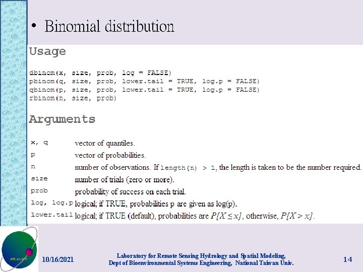
• Binomial distribution 10/16/2021 Laboratory for Remote Sensing Hydrology and Spatial Modeling, Dept of Bioenvironmental Systems Engineering, National Taiwan Univ. 14

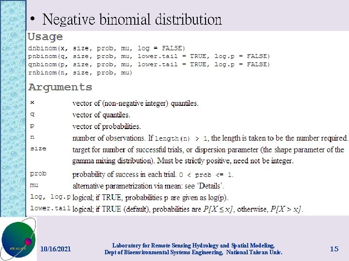
• Negative binomial distribution 10/16/2021 Laboratory for Remote Sensing Hydrology and Spatial Modeling, Dept of Bioenvironmental Systems Engineering, National Taiwan Univ. 15

• Geometric distribution 10/16/2021 Laboratory for Remote Sensing Hydrology and Spatial Modeling, Dept of Bioenvironmental Systems Engineering, National Taiwan Univ. 16

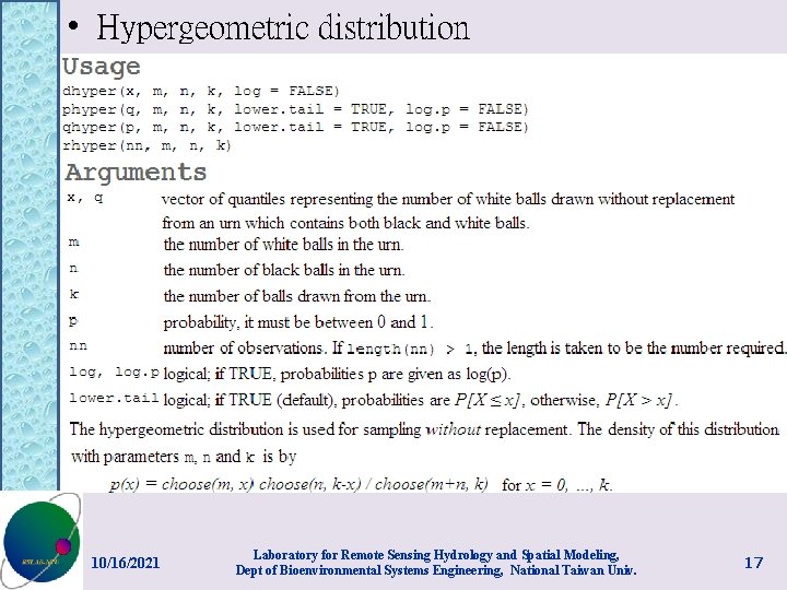
• Hypergeometric distribution 10/16/2021 Laboratory for Remote Sensing Hydrology and Spatial Modeling, Dept of Bioenvironmental Systems Engineering, National Taiwan Univ. 17

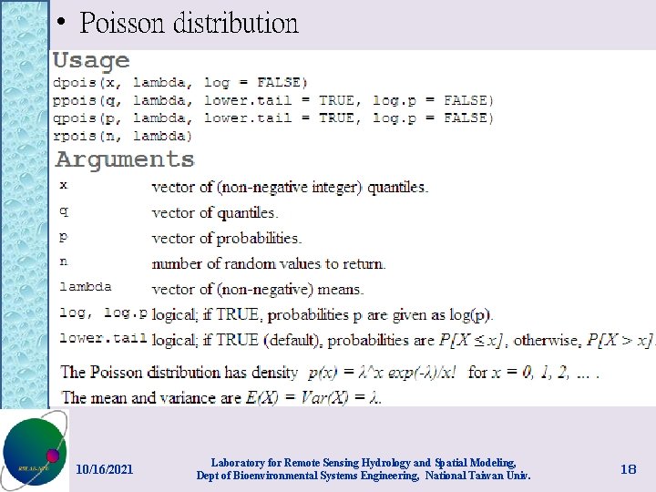
• Poisson distribution 10/16/2021 Laboratory for Remote Sensing Hydrology and Spatial Modeling, Dept of Bioenvironmental Systems Engineering, National Taiwan Univ. 18

An example of stochastic simulation • The travel time from your home (or dormitory) to NTU campus may involve a few factors: – Walking to bus stop (stop for traffic lights, crowdedness on the streets, etc. ) – Transportation by bus – Stop by 7 -11 or Starbucks for breakfast (long queue) – Walking to campus 10/16/2021 Lab for Remote Sensing Hydrology and Spatial Modeling Dept of Bioenvironmental Systems Engineering, NTU 19

Gamma distribution with mean 30 minutes and standard deviation 10 minutes. Exponential distribution with a mean of 20 minutes. All Xi’s are independently distributed. • If you leave home at 8: 00 a. m. for a class session of 9: 10, what is the probability of being late for the class? 10/16/2021 Lab for Remote Sensing Hydrology and Spatial Modeling Dept of Bioenvironmental Systems Engineering, NTU 20

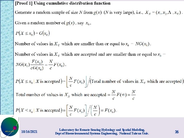
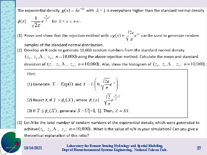
The Acceptance/Rejection Method • This method uses an auxiliary density for generation of random quantities from another distribution. This method is particularly useful for generating random numbers of random variables whose cumulative distribution functions cannot be expressed in closed form. 10/16/2021 Lab for Remote Sensing Hydrology and Spatial Modeling Dept of Bioenvironmental Systems Engineering, NTU 21

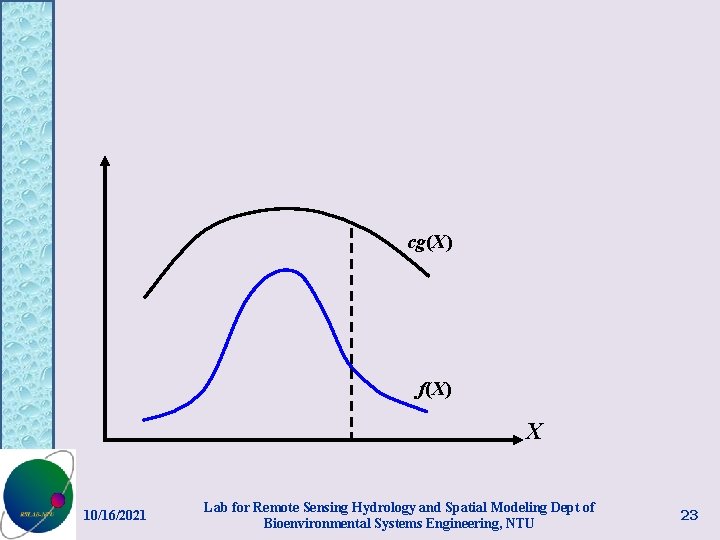
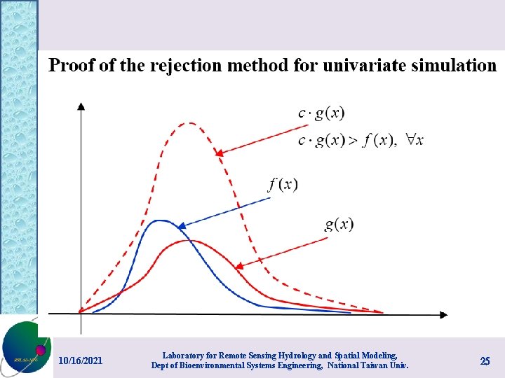
• Suppose that we want to generate random numbers of a random variable X with density f(X). • An auxiliary density g(X) which we know how to generate random samples is identified and cg(X) is everywhere no less than f(X) for some constant c, i. e. , 10/16/2021 Lab for Remote Sensing Hydrology and Spatial Modeling Dept of Bioenvironmental Systems Engineering, NTU 22

cg(X) f(X) X 10/16/2021 Lab for Remote Sensing Hydrology and Spatial Modeling Dept of Bioenvironmental Systems Engineering, NTU 23

• • Generate a random number x of density g(X), Generate a random number u from the density U[0, cg(x)), Reject x if u > f(x); otherwise, x is accepted as a random number from f(X), Repeat the above steps until the desired number of random numbers are obtained. 10/16/2021 Lab for Remote Sensing Hydrology and Spatial Modeling Dept of Bioenvironmental Systems Engineering, NTU 24

10/16/2021 Laboratory for Remote Sensing Hydrology and Spatial Modeling, Dept of Bioenvironmental Systems Engineering, National Taiwan Univ. 25

10/16/2021 Laboratory for Remote Sensing Hydrology and Spatial Modeling, Dept of Bioenvironmental Systems Engineering, National Taiwan Univ. 26

10/16/2021 Laboratory for Remote Sensing Hydrology and Spatial Modeling, Dept of Bioenvironmental Systems Engineering, National Taiwan Univ. 27