Simulation and Modelling 7 Simulation of Inventory Systems

Simulation and Modelling (7) Simulation of Inventory Systems Prof. Moheb Ramzy Girgis Department of Computer Science Faculty of Science Minia University

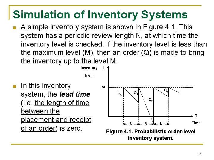
Simulation of Inventory Systems n A simple inventory system is shown in Figure 4. 1. This system has a periodic review length N, at which time the inventory level is checked. If the inventory level is less than the maximum level (M), then an order (Q) is made to bring the inventory up to the level M. Inventory I Level n In this inventory system, the lead time (i. e. the length of time between the placement and receipt of an order) is zero. M Q 3 Q 1 Q 2 T N N N Time Figure 4. 1. Probabilistic order-level inventory system. 2

Simulation of Inventory Systems n …Since demands are not usually known with certainty, the n n n order quantities are probabilistic. At a review point, if the amount in inventory was below zero, indicating a shortage, then these units are backordered. When the order arrives, the demand for the backordered items is satisfied first. To avoid shortage, a safety stock would need to be kept. Keeping stock in inventory has associated costs such as: q The interests on the funds borrowed to buy the items. q Stock holding costs: renting of storage space, hiring guards, and so on. An alternative to keeping high inventory is to make more frequent reviews, and consequently, more frequent purchases. This has an associated cost: the ordering cost. 3

Simulation of Inventory Systems n …Also, there is a cost in being short: Customers n n may get angry, with a subsequent loss of good will. These costs must be traded off in order to minimize the total cost of an inventory system. The total cost (or total profit) of an inventory system is its measure of performance. This can be affected by the policy alternatives, such as controlling: q the maximum inventory level, M, and q the length of the review period (cycle), N. 4

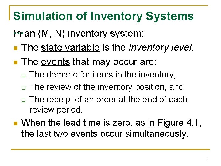
Simulation of Inventory Systems … In an (M, N) inventory system: n n The state variable is the inventory level. The events that may occur are: q q q n The demand for items in the inventory, The review of the inventory position, and The receipt of an order at the end of each review period. When the lead time is zero, as in Figure 4. 1, the last two events occur simultaneously. 5

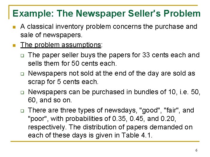
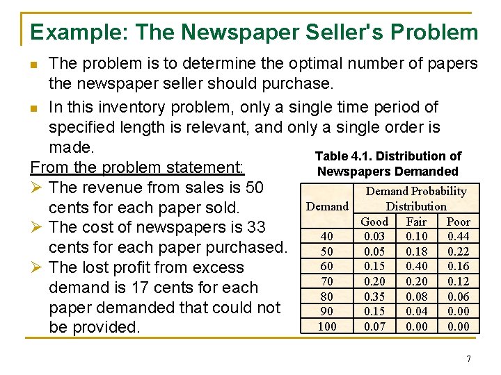
Example: The Newspaper Seller's Problem n n A classical inventory problem concerns the purchase and sale of newspapers. The problem assumptions: q The paper seller buys the papers for 33 cents each and sells them for 50 cents each. q Newspapers not sold at the end of the day are sold as scrap for 5 cents each. q Newspapers can be purchased in bundles of 10, i. e. 50, 60, and so on. q There are three types of newsdays, "good", "fair", and "poor", with probabilities of 0. 35, 0. 45, and 0. 20, respectively. The distribution of papers demanded on each of these days is given in Table 4. 1. 6

Example: The Newspaper Seller's Problem The problem is to determine the optimal number of papers the newspaper seller should purchase. n In this inventory problem, only a single time period of specified length is relevant, and only a single order is made. Table 4. 1. Distribution of From the problem statement: Newspapers Demanded Ø The revenue from sales is 50 Demand Probability Distribution Demand cents for each paper sold. Good Fair Poor Ø The cost of newspapers is 33 40 0. 03 0. 10 0. 44 cents for each paper purchased. 50 0. 05 0. 18 0. 22 60 0. 15 0. 40 0. 16 Ø The lost profit from excess 70 0. 20 0. 12 demand is 17 cents for each 80 0. 35 0. 08 0. 06 paper demanded that could not 90 0. 15 0. 04 0. 00 100 0. 07 0. 00 be provided. n 7

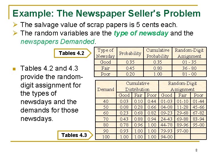
Example: The Newspaper Seller's Problem Ø The salvage value of scrap papers is 5 cents each. Ø The random variables are the type of newsday and the newspapers Demanded. Tables 4. 2 n Tables 4. 2 and 4. 3 provide the randomdigit assignment for the types of newsdays and the demands for those newsdays. Tables 4. 3 Type of Probability Newsday Good 0. 35 Fair 0. 45 Poor 0. 20 Cumulative Probability 0. 35 0. 80 1. 00 Cumulative Demand Distribution Good Fair Poor 40 0. 03 0. 10 0. 44 50 0. 08 0. 28 0. 66 60 0. 23 0. 68 0. 82 70 0. 43 0. 88 0. 94 80 0. 78 0. 96 1. 00 90 0. 93 1. 00 100 1. 00 Random-Digit Assignment 01 - 35 36 - 80 81 - 00 Random-Digit Assignment Good Fair Poor 01 -03 01 -10 01 -44 04 -08 11 -28 45 -66 09 -23 29 -68 67 -82 24 -43 69 -88 83 -94 44 -78 89 -96 95 -00 79 -93 97 -00 94 -00 8

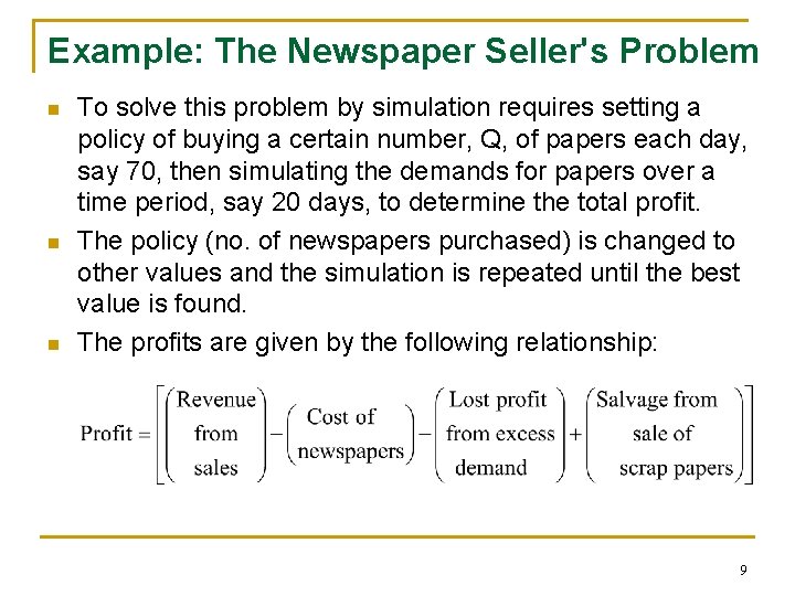
Example: The Newspaper Seller's Problem n n n To solve this problem by simulation requires setting a policy of buying a certain number, Q, of papers each day, say 70, then simulating the demands for papers over a time period, say 20 days, to determine the total profit. The policy (no. of newspapers purchased) is changed to other values and the simulation is repeated until the best value is found. The profits are given by the following relationship: 9

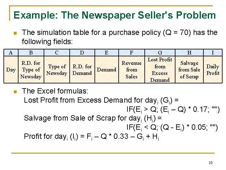
Example: The Newspaper Seller's Problem n A The simulation table for a purchase policy (Q = 70) has the following fields: B C D E F R. D. for Revenue Type of R. D. for Day Type of Demand from Newsday Demand Newsday Sales n G Lost Profit from Excess Demand H I Salvage from Sale of Scrap Daily Profit The Excel formulas: Lost Profit from Excess Demand for dayi (Gi) = IF(Ei > Q; (Ei – Q) * 0. 17; "") Salvage from Sale of Scrap for dayi (Hi) = IF(Ei < Q; (Q - Ei) * 0. 05; "") Profit for dayi (Ii) = Fi – Q * 0. 33 – Gi + Hi 10

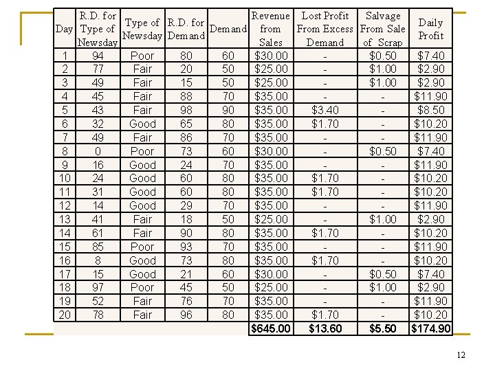
Day 1 2 3 4 5 6 7 8 9 10 11 12 13 14 15 16 17 18 19 20 R. D. for Type of Newsday 94 77 49 45 43 32 49 0 16 24 31 14 41 61 85 8 15 97 52 78 Type of R. D. for Demand Newsday Demand Poor Fair Good Fair Poor Good Poor Fair 80 20 15 88 98 65 86 73 24 60 60 29 18 90 93 73 21 45 76 96 60 50 50 70 90 80 70 60 70 80 80 70 50 80 70 80 60 50 70 80 Revenue Lost Profit Salvage from From Excess From Sales Demand of Scrap $30. 00 $0. 50 $25. 00 $1. 00 $35. 00 $3. 40 $35. 00 $1. 70 $35. 00 $30. 00 $0. 50 $35. 00 $1. 70 $35. 00 $25. 00 $1. 00 $35. 00 $1. 70 $30. 00 $0. 50 $25. 00 $1. 00 $35. 00 $1. 70 $645. 00 $13. 60 $5. 50 Daily Profit $7. 40 $2. 90 $11. 90 $8. 50 $10. 20 $11. 90 $7. 40 $11. 90 $10. 20 $11. 90 $2. 90 $10. 20 $11. 90 $10. 20 $7. 40 $2. 90 $11. 90 $10. 20 $174. 90 11

Day 1 2 3 4 5 6 7 8 9 10 11 12 13 14 15 16 17 18 19 20 R. D. for Type of Newsday 94 77 49 45 43 32 49 0 16 24 31 14 41 61 85 8 15 97 52 78 Type of R. D. for Demand Newsday Demand Poor Fair Good Fair Poor Good Poor Fair 80 20 15 88 98 65 86 73 24 60 60 29 18 90 93 73 21 45 76 96 60 50 50 70 90 80 70 60 70 80 80 70 50 80 70 80 60 50 70 80 Revenue Lost Profit Salvage from From Excess From Sales Demand of Scrap $30. 00 $0. 50 $25. 00 $1. 00 $35. 00 $3. 40 $35. 00 $1. 70 $35. 00 $30. 00 $0. 50 $35. 00 $1. 70 $35. 00 $25. 00 $1. 00 $35. 00 $1. 70 $30. 00 $0. 50 $25. 00 $1. 00 $35. 00 $1. 70 $645. 00 $13. 60 $5. 50 Daily Profit $7. 40 $2. 90 $11. 90 $8. 50 $10. 20 $11. 90 $7. 40 $11. 90 $10. 20 $11. 90 $2. 90 $10. 20 $11. 90 $10. 20 $7. 40 $2. 90 $11. 90 $10. 20 $174. 90 12

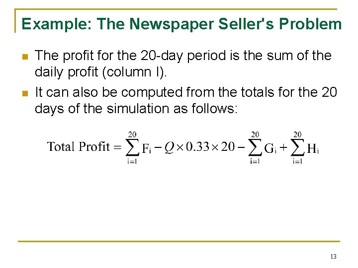
Example: The Newspaper Seller's Problem n n The profit for the 20 -day period is the sum of the daily profit (column I). It can also be computed from the totals for the 20 days of the simulation as follows: 13