Simulation and Modelling 3 Examples of Queueing Systems

Simulation and Modelling (3) Examples of Queueing Systems Simulation Prof. Moheb Ramzy Girgis Department of Computer Science Faculty of Science Minia University

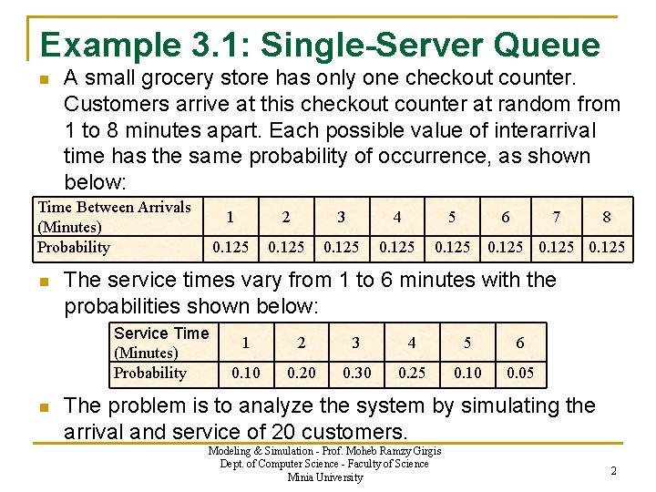
Example 3. 1: Single-Server Queue n A small grocery store has only one checkout counter. Customers arrive at this checkout counter at random from 1 to 8 minutes apart. Each possible value of interarrival time has the same probability of occurrence, as shown below: Time Between Arrivals (Minutes) Probability n 2 3 4 5 0. 125 6 7 8 0. 125 The service times vary from 1 to 6 minutes with the probabilities shown below: Service Time (Minutes) Probability n 1 1 2 3 4 5 6 0. 10 0. 20 0. 30 0. 25 0. 10 0. 05 The problem is to analyze the system by simulating the arrival and service of 20 customers. Modeling & Simulation - Prof. Moheb Ramzy Girgis Dept. of Computer Science - Faculty of Science Minia University 2

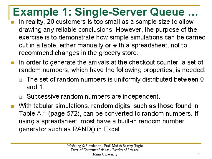
Example 1: Single-Server Queue … n n n In reality, 20 customers is too small as a sample size to allow drawing any reliable conclusions. However, the purpose of the exercise is to demonstrate how simple simulations can be carried out in a table, either manually or with a spreadsheet, not to recommend changes in the grocery store. In order to generate the arrivals at the checkout counter, a set of random numbers, which have the following properties, is needed: q The set of random numbers is uniformly distributed between 0 and 1. q Successive random numbers are independent. With tabular simulations, random digits, such as those found in Table A. 1 (page 572), can be converted to random numbers. If using a spreadsheet, most have a built-in random number generator such as RAND() in Excel. Modeling & Simulation - Prof. Moheb Ramzy Girgis Dept. of Computer Science - Faculty of Science Minia University 3

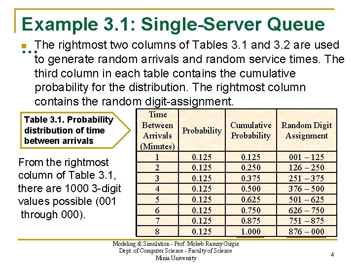
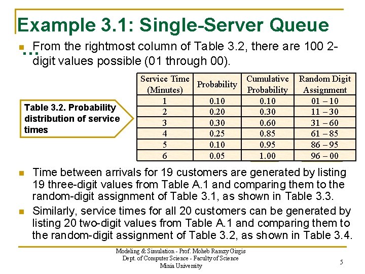
Example 3. 1: Single-Server Queue n The rightmost two columns of Tables 3. 1 and 3. 2 are used … to generate random arrivals and random service times. The third column in each table contains the cumulative probability for the distribution. The rightmost column contains the random digit-assignment. Table 3. 1. Probability distribution of time between arrivals From the rightmost column of Table 3. 1, there are 1000 3 -digit values possible (001 through 000). Time Between Cumulative Probability Arrivals Probability (Minutes) 1 0. 125 2 0. 125 0. 250 3 0. 125 0. 375 4 0. 125 0. 500 5 0. 125 0. 625 6 0. 125 0. 750 7 0. 125 0. 875 8 0. 125 1. 000 Modeling & Simulation - Prof. Moheb Ramzy Girgis Dept. of Computer Science - Faculty of Science Minia University Random Digit Assignment 001 – 125 126 – 250 251 – 375 376 – 500 501 – 625 626 – 750 751 – 875 876 – 000 4

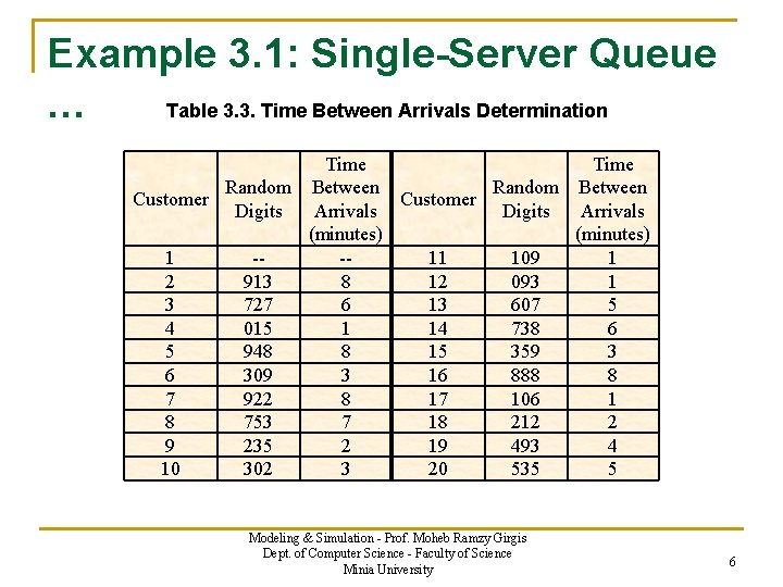
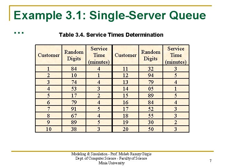
Example 3. 1: Single-Server Queue n From the rightmost column of Table 3. 2, there are 100 2… digit values possible (01 through 00). Table 3. 2. Probability distribution of service times n n Service Time Cumulative Probability (Minutes) Probability 1 0. 10 2 0. 20 0. 30 3 0. 30 0. 60 4 0. 25 0. 85 5 0. 10 0. 95 6 0. 05 1. 00 Random Digit Assignment 01 – 10 11 – 30 31 – 60 61 – 85 86 – 95 96 – 00 Time between arrivals for 19 customers are generated by listing 19 three-digit values from Table A. 1 and comparing them to the random-digit assignment of Table 3. 1, as shown in Table 3. 3. Similarly, service times for all 20 customers can be generated by listing 20 two-digit values from Table A. 1 and comparing them to the random-digit assignment of Table 3. 2, as shown in Table 3. 4. Modeling & Simulation - Prof. Moheb Ramzy Girgis Dept. of Computer Science - Faculty of Science Minia University 5

Example 3. 1: Single-Server Queue … Table 3. 3. Time Between Arrivals Determination Time Random Between Customer Digits Arrivals (minutes) 1 --11 109 1 2 913 8 12 093 1 3 727 6 13 607 5 4 015 1 14 738 6 5 948 8 15 359 3 6 309 3 16 888 8 7 922 8 17 106 1 8 753 7 18 212 2 9 235 2 19 493 4 10 302 3 20 535 5 Modeling & Simulation - Prof. Moheb Ramzy Girgis Dept. of Computer Science - Faculty of Science Minia University 6

Example 3. 1: Single-Server Queue … Table 3. 4. Service Times Determination Random Customer Digits 1 2 3 4 5 6 7 8 9 10 84 10 74 53 17 79 91 67 89 38 Service Random Time Customer Digits (minutes) 4 11 32 3 1 12 94 5 4 13 79 4 3 14 05 1 2 15 89 5 4 16 84 4 5 17 52 3 4 18 55 3 5 19 30 2 3 20 50 3 Modeling & Simulation - Prof. Moheb Ramzy Girgis Dept. of Computer Science - Faculty of Science Minia University 7

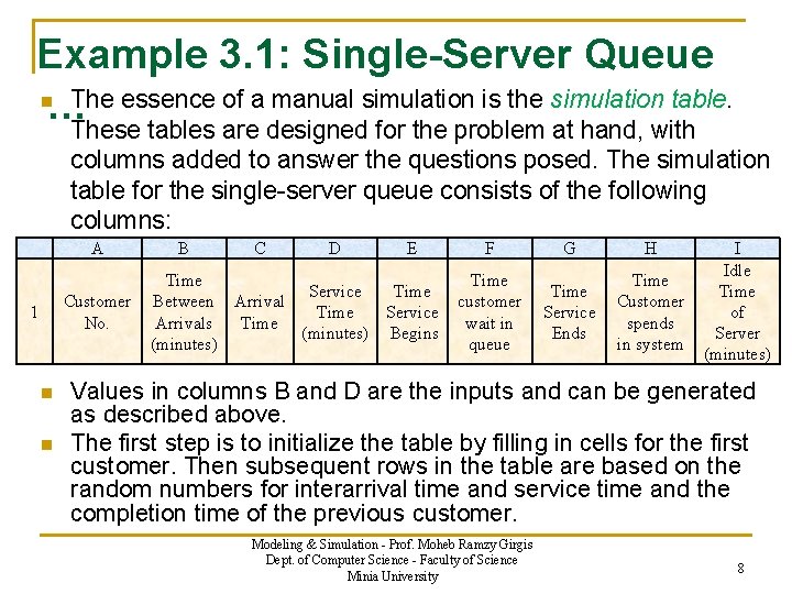
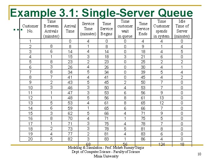
Example 3. 1: Single-Server Queue n The essence of a manual simulation is the simulation table. …These tables are designed for the problem at hand, with columns added to answer the questions posed. The simulation table for the single-server queue consists of the following columns: A Customer No. 1 n n B C D E Time Service Time Between Arrival Time Service Arrivals Time (minutes) Begins (minutes) F G H Time customer wait in queue Time Service Ends Time Customer spends in system I Idle Time of Server (minutes) Values in columns B and D are the inputs and can be generated as described above. The first step is to initialize the table by filling in cells for the first customer. Then subsequent rows in the table are based on the random numbers for interarrival time and service time and the completion time of the previous customer. Modeling & Simulation - Prof. Moheb Ramzy Girgis Dept. of Computer Science - Faculty of Science Minia University 8

Example 3. 1: Single-Server Queue … Customer No. 1 2 3 4 5 6 7 8 9 10 11 12 13 14 15 16 17 18 19 20 Time Between Arrivals (minutes) 8 6 1 8 3 8 7 2 3 1 1 5 6 3 8 1 2 4 5 Service Arrival Time (minutes) 0 8 14 15 23 26 34 41 43 46 47 48 53 59 62 70 71 73 77 82 4 1 4 3 2 4 5 3 3 5 4 1 5 4 3 3 2 3 68 Time Service Begins 0 8 14 18 23 26 34 41 45 50 53 56 61 65 66 71 75 78 81 83 Time customer Service wait Ends in queue 0 4 0 9 0 18 3 21 0 25 0 30 0 39 0 45 2 50 4 53 6 56 8 61 8 65 6 66 4 71 1 75 4 78 5 81 4 83 1 86 56 Modeling & Simulation - Prof. Moheb Ramzy Girgis Dept. of Computer Science - Faculty of Science Minia University Time Customer spends in system 4 1 4 6 2 4 5 4 7 7 9 13 12 7 9 5 7 8 6 4 124 Idle Time of Server (minutes) 0 4 5 0 2 1 4 2 0 0 0 18 9

Example 3. 1: Single-Server Queue … Customer No. 1 2 3 4 5 6 7 8 9 10 11 12 13 14 15 16 17 18 19 20 Time Between Arrivals (minutes) 8 6 1 8 3 8 7 2 3 1 1 5 6 3 8 1 2 4 5 Service Arrival Time (minutes) 0 8 14 15 23 26 34 41 43 46 47 48 53 59 62 70 71 73 77 82 4 1 4 3 2 4 5 3 3 5 4 1 5 4 3 3 2 3 68 Time Service Begins 0 8 14 18 23 26 34 41 45 50 53 56 61 65 66 71 75 78 81 83 Time customer Service wait Ends in queue 0 4 0 9 0 18 3 21 0 25 0 30 0 39 0 45 2 50 4 53 6 56 8 61 8 65 6 66 4 71 1 75 4 78 5 81 4 83 1 86 56 Modeling & Simulation - Prof. Moheb Ramzy Girgis Dept. of Computer Science - Faculty of Science Minia University Time Customer spends in system 4 1 4 6 2 4 5 4 7 7 9 13 12 7 9 5 7 8 6 4 124 Idle Time of Server (minutes) 0 4 5 0 2 1 4 2 0 0 0 18 10

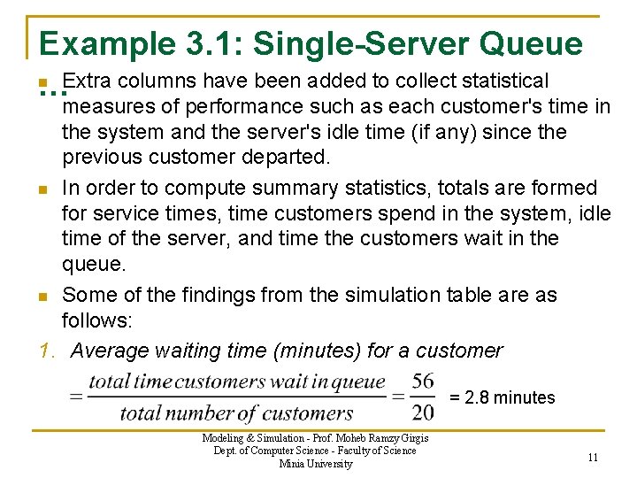
Example 3. 1: Single-Server Queue n Extra columns have been added to collect statistical … measures of performance such as each customer's time in the system and the server's idle time (if any) since the previous customer departed. n In order to compute summary statistics, totals are formed for service times, time customers spend in the system, idle time of the server, and time the customers wait in the queue. n Some of the findings from the simulation table are as follows: 1. Average waiting time (minutes) for a customer = 2. 8 minutes Modeling & Simulation - Prof. Moheb Ramzy Girgis Dept. of Computer Science - Faculty of Science Minia University 11

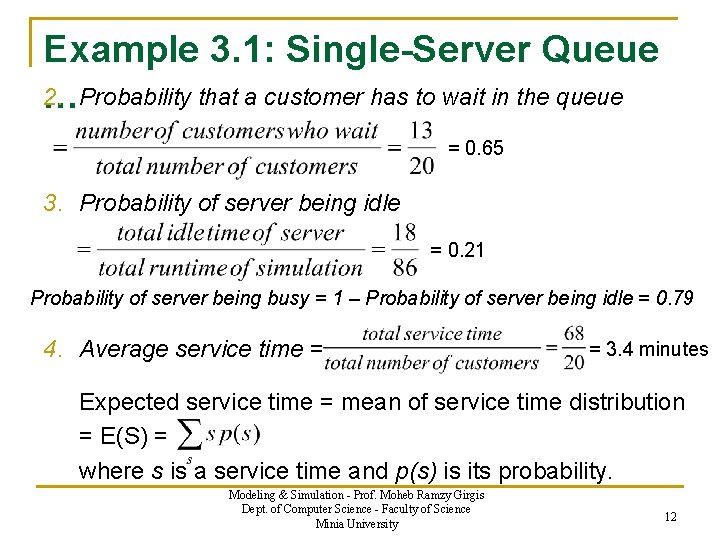
Example 3. 1: Single-Server Queue 2. Probability that a customer has to wait in the queue … = 0. 65 3. Probability of server being idle = 0. 21 Probability of server being busy = 1 – Probability of server being idle = 0. 79 4. Average service time = = 3. 4 minutes Expected service time = mean of service time distribution = E(S) = where s is a service time and p(s) is its probability. Modeling & Simulation - Prof. Moheb Ramzy Girgis Dept. of Computer Science - Faculty of Science Minia University 12

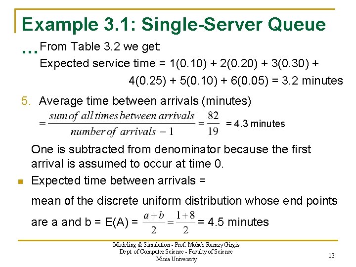
Example 3. 1: Single-Server Queue …From Table 3. 2 we get: Expected service time = 1(0. 10) + 2(0. 20) + 3(0. 30) + 4(0. 25) + 5(0. 10) + 6(0. 05) = 3. 2 minutes 5. Average time between arrivals (minutes) = 4. 3 minutes n One is subtracted from denominator because the first arrival is assumed to occur at time 0. Expected time between arrivals = mean of the discrete uniform distribution whose end points are a and b = E(A) = = 4. 5 minutes Modeling & Simulation - Prof. Moheb Ramzy Girgis Dept. of Computer Science - Faculty of Science Minia University 13

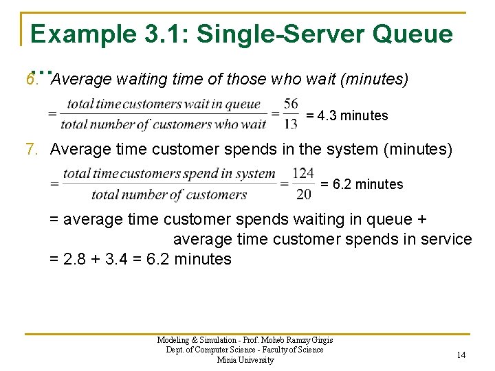
Example 3. 1: Single-Server Queue … 6. Average waiting time of those who wait (minutes) = 4. 3 minutes 7. Average time customer spends in the system (minutes) = 6. 2 minutes = average time customer spends waiting in queue + average time customer spends in service = 2. 8 + 3. 4 = 6. 2 minutes Modeling & Simulation - Prof. Moheb Ramzy Girgis Dept. of Computer Science - Faculty of Science Minia University 14

Example 3. 1: Single-Server Queue C omments on the results of Example 3. 1: … n n A decision maker would be interested in results of this type, but a longer simulation would increase the accuracy of the findings. However, some subjective inferences can be drawn at this point: q q n Most customers have to wait; however, the average waiting time is not excessive. The server does not have an undue amount of idle time. Objective statements about the results would depend on balancing the cost of waiting with the cost of additional servers. Modeling & Simulation - Prof. Moheb Ramzy Girgis Dept. of Computer Science - Faculty of Science Minia University 15

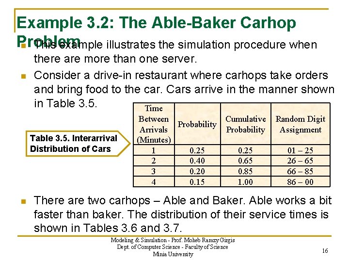
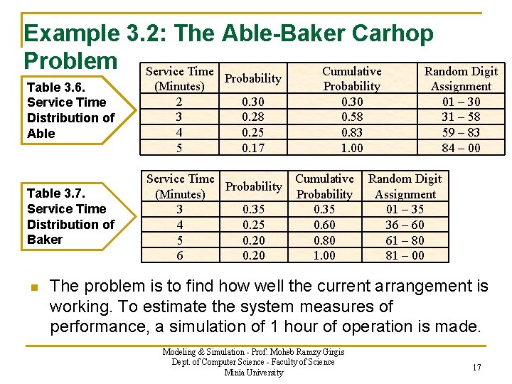
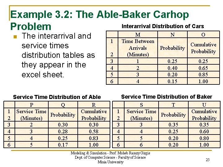
Example 3. 2: The Able-Baker Carhop Problem n This example illustrates the simulation procedure when n there are more than one server. Consider a drive-in restaurant where carhops take orders and bring food to the car. Cars arrive in the manner shown in Table 3. 5. Time Table 3. 5. Interarrival Distribution of Cars n Between Cumulative Probability Arrivals Probability (Minutes) 1 0. 25 2 0. 40 0. 65 3 0. 20 0. 85 4 0. 15 1. 00 Random Digit Assignment 01 – 25 26 – 65 66 – 85 86 – 00 There are two carhops – Able and Baker. Able works a bit faster than baker. The distribution of their service times is shown in Tables 3. 6 and 3. 7. Modeling & Simulation - Prof. Moheb Ramzy Girgis Dept. of Computer Science - Faculty of Science Minia University 16

Example 3. 2: The Able-Baker Carhop Problem Service Time Cumulative Random Digit Table 3. 6. Service Time Distribution of Able Table 3. 7. Service Time Distribution of Baker n (Minutes) 2 3 4 5 Probability 0. 30 0. 28 0. 25 0. 17 Probability 0. 30 0. 58 0. 83 1. 00 Service Time Cumulative Probability (Minutes) Probability 3 0. 35 4 0. 25 0. 60 5 0. 20 0. 80 6 0. 20 1. 00 Assignment 01 – 30 31 – 58 59 – 83 84 – 00 Random Digit Assignment 01 – 35 36 – 60 61 – 80 81 – 00 The problem is to find how well the current arrangement is working. To estimate the system measures of performance, a simulation of 1 hour of operation is made. Modeling & Simulation - Prof. Moheb Ramzy Girgis Dept. of Computer Science - Faculty of Science Minia University 17

Example 3. 2: The Able-Baker Carhop Problem n The simulation proceeds in a manner similar to n n Example 3. 1, except that it is more complex because of the two servers. A simplifying rule is that Able gets the customer if both carhops are idle. Perhaps, Able has seniority. (The simulation would be different if the decision were made at random or by any other rule). Here there are more events: q a customer arrives, q a customer completes service from Able, and q a customer completes service from Baker. Modeling & Simulation - Prof. Moheb Ramzy Girgis Dept. of Computer Science - Faculty of Science Minia University 18

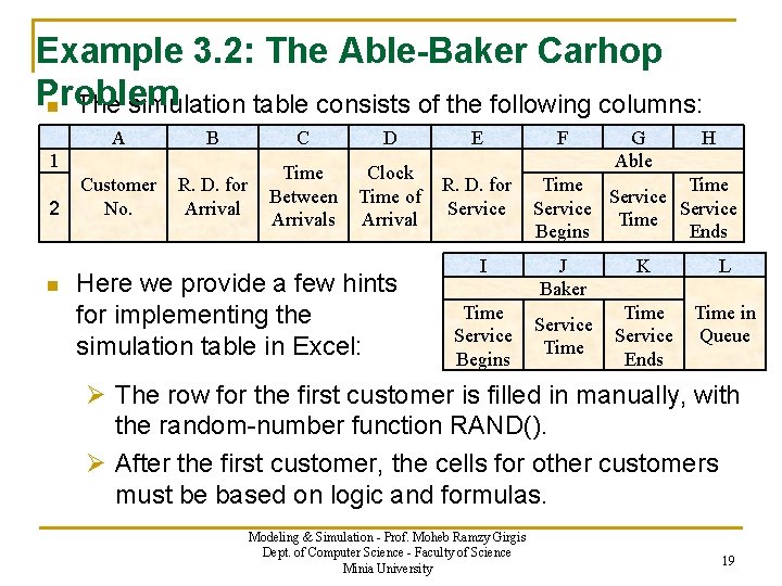
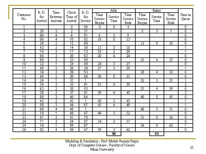
Example 3. 2: The Able-Baker Carhop Problem n The simulation table consists of the following columns: A B C D E Customer No. R. D. for Arrival Time Between Arrivals Clock Time of Arrival R. D. for Service 1 2 n Here we provide a few hints for implementing the simulation table in Excel: I Time Service Begins F G Able H Time Service Time Begins Ends J Baker Service Time K L Time Service Ends Time in Queue Ø The row for the first customer is filled in manually, with the random-number function RAND(). Ø After the first customer, the cells for other customers must be based on logic and formulas. Modeling & Simulation - Prof. Moheb Ramzy Girgis Dept. of Computer Science - Faculty of Science Minia University 19

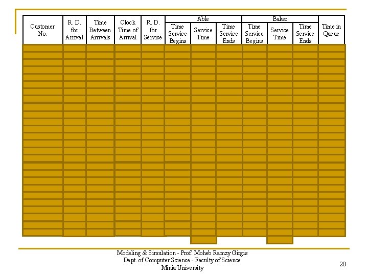
Customer No. 1 2 3 4 5 6 7 8 9 10 11 12 13 14 15 16 17 18 19 20 21 22 23 24 25 26 R. D. for Arrival 26 98 90 26 42 74 80 68 22 48 34 45 24 34 63 38 80 42 56 89 18 51 71 16 92 Time Between Arrivals Clock Time of Arrival R. D. for Service 2 4 4 2 2 3 3 3 1 2 2 2 3 2 2 4 1 2 3 1 4 0 2 6 10 12 14 17 20 23 24 26 28 30 31 33 35 37 40 42 44 48 49 51 54 55 59 95 21 51 92 89 38 13 62 50 49 39 53 88 1 81 53 81 64 1 67 1 47 75 57 87 47 Able Time Service Begins 0 Baker 5 Time Service Ends 5 6 10 3 5 9 15 15 18 20 3 2 4 18 20 24 Service Time 24 27 3 3 27 30 30 5 35 35 39 43 45 49 4 4 2 4 3 Time Service Begins Service Time Service Ends 2 3 5 12 6 18 23 4 27 28 4 32 32 3 35 35 4 39 40 5 45 48 3 51 51 5 56 56 6 62 39 43 45 49 52 54 3 57 59 3 56 62 Modeling & Simulation - Prof. Moheb Ramzy Girgis Dept. of Computer Science - Faculty of Science Minia University Time in Queue 0 0 0 1 1 0 0 0 1 2 0 1 1 0 0 1 0 43 20

Customer No. 1 2 3 4 5 6 7 8 9 10 11 12 13 14 15 16 17 18 19 20 21 22 23 24 25 26 R. D. for Arrival 26 98 90 26 42 74 80 68 22 48 34 45 24 34 63 38 80 42 56 89 18 51 71 16 92 Time Between Arrivals Clock Time of Arrival R. D. for Service 2 4 4 2 2 3 3 3 1 2 2 2 3 2 2 4 1 2 3 1 4 0 2 6 10 12 14 17 20 23 24 26 28 30 31 33 35 37 40 42 44 48 49 51 54 55 59 95 21 51 92 89 38 13 62 50 49 39 53 88 1 81 53 81 64 1 67 1 47 75 57 87 47 Able Time Service Begins 0 Baker 5 Time Service Ends 5 6 10 3 5 9 15 15 18 20 3 2 4 18 20 24 Service Time 24 27 3 3 27 30 30 5 35 35 39 43 45 49 4 4 2 4 3 Time Service Begins Service Time Service Ends 2 3 5 12 6 18 23 4 27 28 4 32 32 3 35 35 4 39 40 5 45 48 3 51 51 5 56 56 6 62 39 43 45 49 52 54 3 57 59 3 56 62 Modeling & Simulation - Prof. Moheb Ramzy Girgis Dept. of Computer Science - Faculty of Science Minia University Time in Queue 0 0 0 1 1 0 0 0 1 2 0 1 1 0 0 1 0 43 21

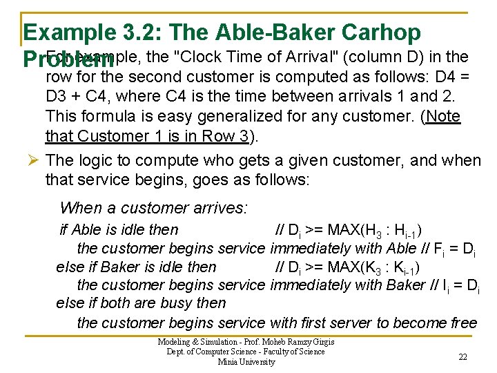
Example 3. 2: The Able-Baker Carhop For example, the "Clock Time of Arrival" (column D) in the Problem row for the second customer is computed as follows: D 4 = D 3 + C 4, where C 4 is the time between arrivals 1 and 2. This formula is easy generalized for any customer. (Note that Customer 1 is in Row 3). Ø The logic to compute who gets a given customer, and when that service begins, goes as follows: When a customer arrives: if Able is idle then // Di >= MAX(H 3 : Hi-1) the customer begins service immediately with Able // Fi = Di else if Baker is idle then // Di >= MAX(K 3 : Ki-1) the customer begins service immediately with Baker // Ii = Di else if both are busy then the customer begins service with first server to become free Modeling & Simulation - Prof. Moheb Ramzy Girgis Dept. of Computer Science - Faculty of Science Minia University 22

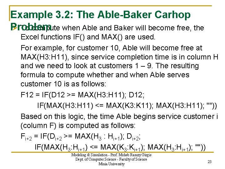
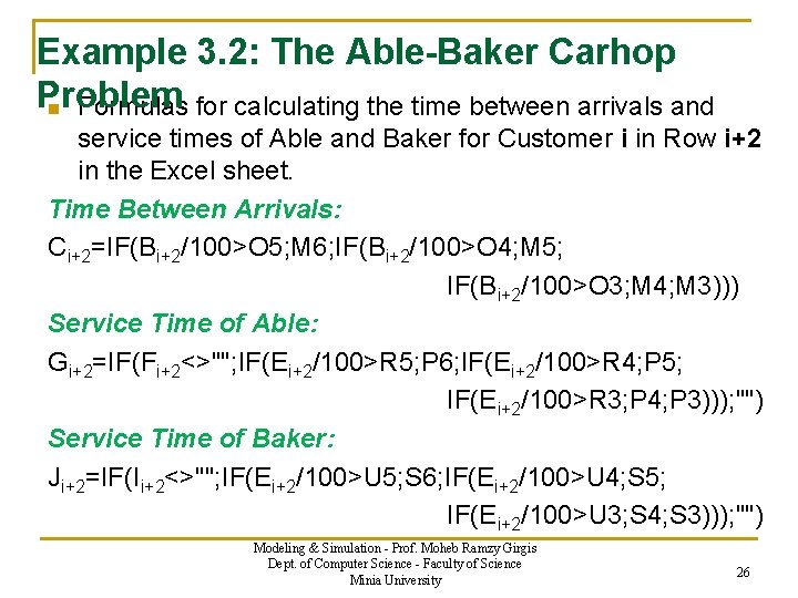
Example 3. 2: The Able-Baker Carhop Problem Ø To compute when Able and Baker will become free, the Excel functions IF() and MAX() are used. For example, for customer 10, Able will become free at MAX(H 3: H 11), since service completion time is in column H and we need to look at customers 1 – 9. The resulting formula to compute whether and when Able serves customer 10 is as follows: F 12 = IF(D 12 >= MAX(H 3: H 11); D 12; IF(MAX(H 3: H 11) <= MAX(K 3: K 11); MAX(H 3: H 11); "")) Based on this logic, the time Able begins service customer i (column F) is computed as follows: Fi+2 = IF(Di+2 >= MAX(H 3 : Hi+1); Di+2; IF(MAX(H 3: Hi+1) <= MAX(K 3: Ki+1); MAX(H 3: Hi+1); "")) Modeling & Simulation - Prof. Moheb Ramzy Girgis Dept. of Computer Science - Faculty of Science Minia University 23

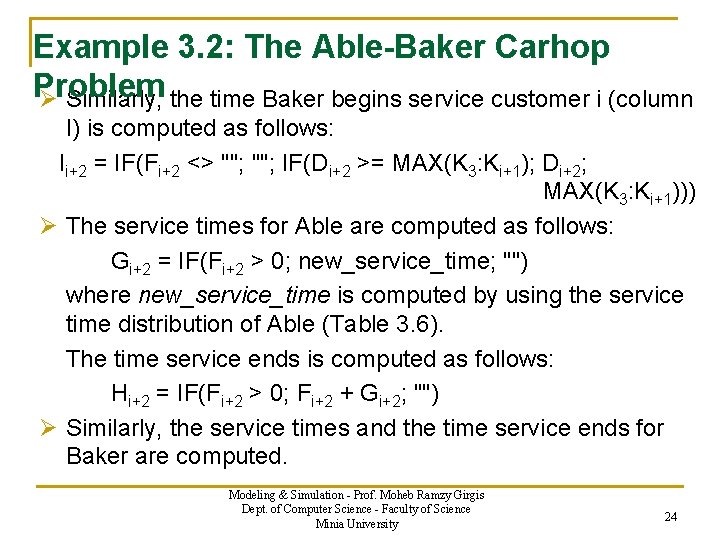
Example 3. 2: The Able-Baker Carhop Problem Ø Similarly, the time Baker begins service customer i (column I) is computed as follows: Ii+2 = IF(Fi+2 <> ""; IF(Di+2 >= MAX(K 3: Ki+1); Di+2; MAX(K 3: Ki+1))) Ø The service times for Able are computed as follows: Gi+2 = IF(Fi+2 > 0; new_service_time; "") where new_service_time is computed by using the service time distribution of Able (Table 3. 6). The time service ends is computed as follows: Hi+2 = IF(Fi+2 > 0; Fi+2 + Gi+2; "") Ø Similarly, the service times and the time service ends for Baker are computed. Modeling & Simulation - Prof. Moheb Ramzy Girgis Dept. of Computer Science - Faculty of Science Minia University 24

Example 3. 2: The Able-Baker Carhop Interarrival Distribution of Cars Problem n 1 2 3 4 5 6 The interarrival and service times distribution tables as they appear in the excel sheet. Service Time Distribution of Able P Q R Service Time Cumulative Probability (Minutes) Probability 2 0. 30 3 0. 28 0. 58 4 0. 25 0. 83 5 0. 17 1. 00 1 2 3 4 5 6 M Time Between Arrivals (Minutes) 1 2 3 4 N O Probability Cumulative Probability 0. 25 0. 40 0. 20 0. 15 0. 25 0. 65 0. 85 1. 00 Service Time Distribution of Baker S T U 1 Service Time Cumulative Probability 2 (Minutes) Probability 3 3 0. 35 4 4 0. 25 0. 60 5 5 0. 20 0. 80 6 6 0. 20 1. 00 Modeling & Simulation - Prof. Moheb Ramzy Girgis Dept. of Computer Science - Faculty of Science Minia University 25

Example 3. 2: The Able-Baker Carhop Problem n Formulas for calculating the time between arrivals and service times of Able and Baker for Customer i in Row i+2 in the Excel sheet. Time Between Arrivals: Ci+2=IF(Bi+2/100>O 5; M 6; IF(Bi+2/100>O 4; M 5; IF(Bi+2/100>O 3; M 4; M 3))) Service Time of Able: Gi+2=IF(Fi+2<>""; IF(Ei+2/100>R 5; P 6; IF(Ei+2/100>R 4; P 5; IF(Ei+2/100>R 3; P 4; P 3))); "") Service Time of Baker: Ji+2=IF(Ii+2<>""; IF(Ei+2/100>U 5; S 6; IF(Ei+2/100>U 4; S 5; IF(Ei+2/100>U 3; S 4; S 3))); "") Modeling & Simulation - Prof. Moheb Ramzy Girgis Dept. of Computer Science - Faculty of Science Minia University 26

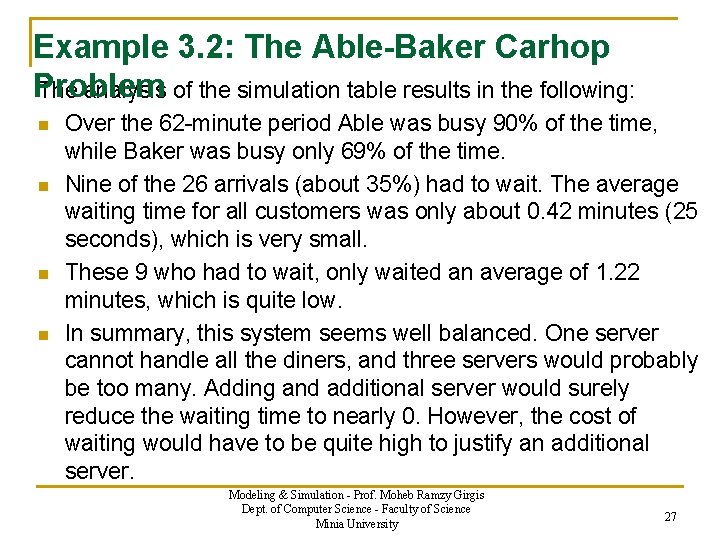
Example 3. 2: The Able-Baker Carhop Problem The analysis of the simulation table results in the following: n n Over the 62 -minute period Able was busy 90% of the time, while Baker was busy only 69% of the time. Nine of the 26 arrivals (about 35%) had to wait. The average waiting time for all customers was only about 0. 42 minutes (25 seconds), which is very small. These 9 who had to wait, only waited an average of 1. 22 minutes, which is quite low. In summary, this system seems well balanced. One server cannot handle all the diners, and three servers would probably be too many. Adding and additional server would surely reduce the waiting time to nearly 0. However, the cost of waiting would have to be quite high to justify an additional server. Modeling & Simulation - Prof. Moheb Ramzy Girgis Dept. of Computer Science - Faculty of Science Minia University 27