Simulating the Nonlinear Schrodinger Equation using MATLAB with

Simulating the Nonlinear Schrodinger Equation using MATLAB with CUDA COMP 670 October 21 st 2009 Eunsil Baik , Ron Caplan, Fred Mc. Donald

Overview Introduction NLS and Soliton Solution Numerical Method CUDA and MATLAB Overview Setup MEX Implementation Code design Results GPUmat Implementation Code design Results Conclusion 2

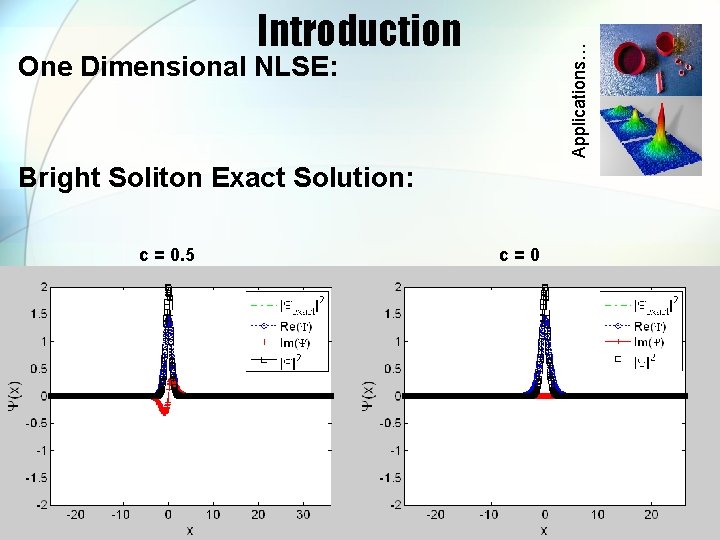
Applications… Introduction One Dimensional NLSE: Bright Soliton Exact Solution: c = 0. 5 c=0

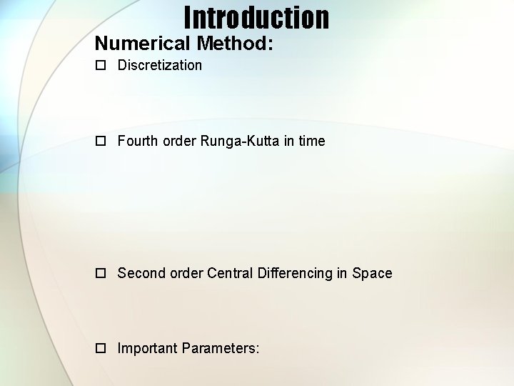
Introduction Numerical Method: Discretization Fourth order Runga-Kutta in time Second order Central Differencing in Space Important Parameters:

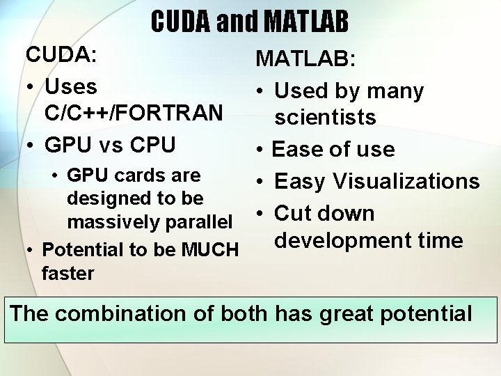
CUDA and MATLAB CUDA: • Uses C/C++/FORTRAN • GPU vs CPU MATLAB: • Used by many scientists • Ease of use • GPU cards are • Easy Visualizations designed to be massively parallel • Cut down development time • Potential to be MUCH faster The combination of both has great potential

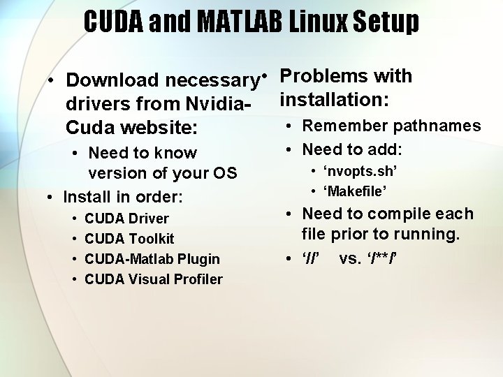
CUDA and MATLAB Linux Setup • Download necessary • Problems with drivers from Nvidia- installation: • Remember pathnames Cuda website: • Need to know version of your OS • Install in order: • • CUDA Driver CUDA Toolkit CUDA-Matlab Plugin CUDA Visual Profiler • Need to add: • ‘nvopts. sh’ • ‘Makefile’ • Need to compile each file prior to running. • ‘//’ vs. ‘/**/’

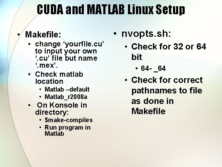
CUDA and MATLAB Linux Setup • Makefile: • change ‘yourfile. cu’ to input your own ‘. cu’ file but name ‘. mex’. • Check matlab location • Matlab –default • Matlab_r 2008 a • On Konsole in directory: • $make-compiles • Run program in Matlab • nvopts. sh: • Check for 32 or 64 bit • 64 - _64 • Check for correct pathnames to file as done in Makefile

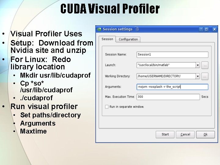
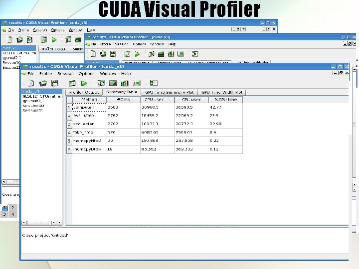
CUDA Visual Profiler • Visual Profiler Uses • Setup: Download from Nvidia site and unzip • For Linux: Redo library location • Mkdir usr/lib/cudaprof • Cp *so* /usr/lib/cudaprof • . /cudaprof • Run visual profiler • Set paths/directory • Arguments • Maxtime

CUDA Visual Profiler

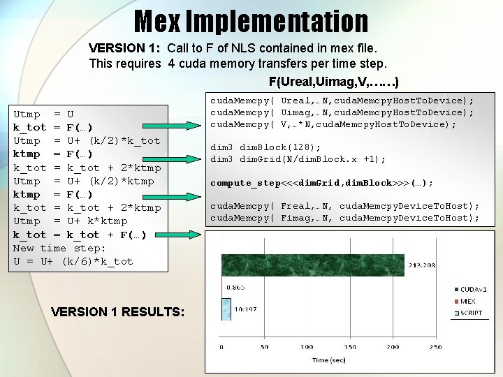
Mex Implementation VERSION 1: Call to F of NLS contained in mex file. This requires 4 cuda memory transfers per time step. F(Ureal, Uimag, V, ……) Utmp = U k_tot = F(…) Utmp = U+ (k/2)*k_tot ktmp = F(…) k_tot = k_tot + 2*ktmp Utmp = U+ (k/2)*ktmp = F(…) k_tot = k_tot + 2*ktmp Utmp = U+ k*ktmp k_tot = k_tot + F(…) New time step: U = U+ (k/6)*k_tot VERSION 1 RESULTS: cuda. Memcpy( Ureal, …N, cuda. Memcpy. Host. To. Device); cuda. Memcpy( Uimag, …N, cuda. Memcpy. Host. To. Device); cuda. Memcpy( V, …*N, cuda. Memcpy. Host. To. Device); dim 3 dim. Block(128); dim 3 dim. Grid(N/dim. Block. x +1); compute_step<<<dim. Grid, dim. Block>>>(…); cuda. Memcpy( Freal, …N, cuda. Memcpy. Device. To. Host); cuda. Memcpy( Fimag, …N, cuda. Memcpy. Device. To. Host);

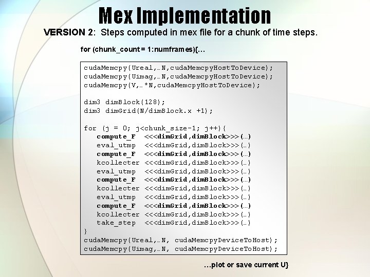
Mex Implementation VERSION 2: Steps computed in mex file for a chunk of time steps. for (chunk_count = 1: numframes){… cuda. Memcpy(Ureal, …N, cuda. Memcpy. Host. To. Device); cuda. Memcpy(Uimag, …N, cuda. Memcpy. Host. To. Device); cuda. Memcpy(V, …*N, cuda. Memcpy. Host. To. Device); dim 3 dim. Block(128); dim 3 dim. Grid(N/dim. Block. x +1); for (j = 0; j<chunk_size-1; j++){ compute_F <<<dim. Grid, dim. Block>>>(…) eval_utmp <<<dim. Grid, dim. Block>>>(…) compute_F <<<dim. Grid, dim. Block>>>(…) kcollecter <<<dim. Grid, dim. Block>>>(…) take_step <<<dim. Grid, dim. Block>>>(…) } cuda. Memcpy(Ureal, …N, cuda. Memcpy. Device. To. Host); cuda. Memcpy(Uimag, …N, cuda. Memcpy. Device. To. Host); …plot or save current U}

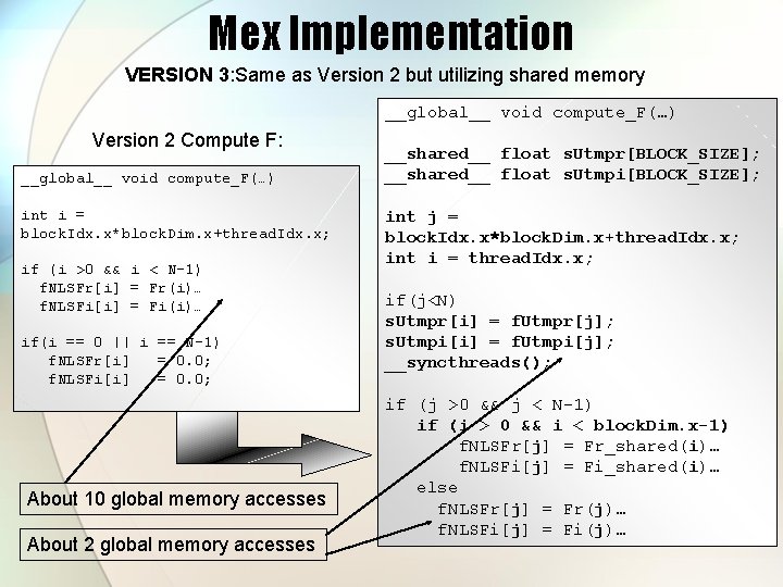
Mex Implementation VERSION 3: Same as Version 2 but utilizing shared memory __global__ void compute_F(…) Version 2 Compute F: __global__ void compute_F(…) int i = block. Idx. x*block. Dim. x+thread. Idx. x; if (i >0 && i < N-1) f. NLSFr[i] = Fr(i)… f. NLSFi[i] = Fi(i)… if(i == 0 || i == N-1) f. NLSFr[i] = 0. 0; f. NLSFi[i] = 0. 0; About 10 global memory accesses About 2 global memory accesses __shared__ float s. Utmpr[BLOCK_SIZE]; __shared__ float s. Utmpi[BLOCK_SIZE]; int j = block. Idx. x*block. Dim. x+thread. Idx. x; int i = thread. Idx. x; if(j<N) s. Utmpr[i] = f. Utmpr[j]; s. Utmpi[i] = f. Utmpi[j]; __syncthreads(); if (j >0 && j < N-1) if (i > 0 && i < block. Dim. x-1) f. NLSFr[j] = Fr_shared(i)… f. NLSFi[j] = Fi_shared(i)… else f. NLSFr[j] = Fr(j)… f. NLSFi[j] = Fi(j)…

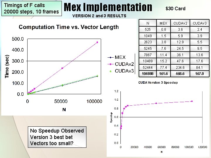
Timings of F calls 20000 steps, 10 frames Mex Implementation $30 Card VERSION 2 and 3 RESULTS No Speedup Observed Version 3 best bet Vectors too small? N MEX CUDAv 2 CUDAv 3 525 0. 8 3. 6 2. 4 1049 1. 5 5. 9 3. 9 2623 3. 8 12. 9 5. 5 5245 7. 6 24. 5 9. 5 7867 11. 4 36. 1 13. 6 10489 15. 2 47. 6 17. 6 52444 77. 4 234. 6 84. 1 104888 161. 6 468. 6 167. 0

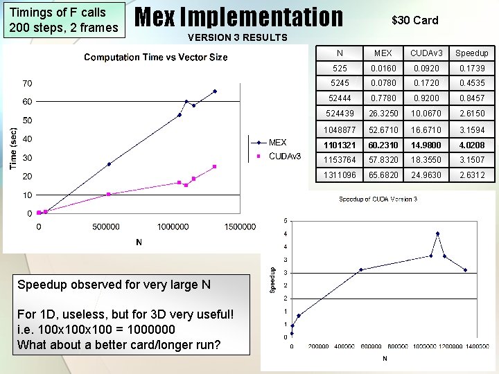
Timings of F calls 200 steps, 2 frames Mex Implementation $30 Card VERSION 3 RESULTS Speedup observed for very large N For 1 D, useless, but for 3 D very useful! i. e. 100 x 100 = 1000000 What about a better card/longer run? N MEX CUDAv 3 Speedup 525 0. 0160 0. 0920 0. 1739 5245 0. 0780 0. 1720 0. 4535 52444 0. 7780 0. 9200 0. 8457 524439 26. 3250 10. 0670 2. 6150 1048877 52. 6710 16. 6710 3. 1594 1101321 60. 2310 14. 9800 4. 0208 1153764 57. 8320 18. 3550 3. 1507 1311096 65. 6820 24. 9630 2. 6312

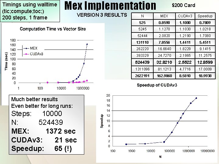
Timings using walltime (tic; compute; toc; ) 200 steps, 1 frame Mex Implementation VERSION 3 RESULTS Much better results Even better for long runs: Steps: 10000 N: 524439 MEX: 1372 sec CUDAv 3: 21 sec Speedup: 65 (!) $200 Card N MEX CUDAv 3 Speedup 525 0. 8590 1. 1000 0. 7809 5245 1. 1270 1. 1030 1. 0218 52444 2. 0820 1. 2190 1. 7080 131110 7. 8556 1. 4411 5. 4511 262220 16. 6640 1. 8229 9. 1415 393329 24. 7270 2. 1965 11. 2575 524439 32. 8210 2. 5522 12. 8599 1311096 81. 1213 4. 7716 17. 0009 2622191 162. 9860 8. 5810 18. 9938

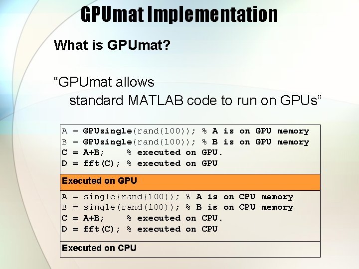
GPUmat Implementation What is GPUmat? “GPUmat allows standard MATLAB code to run on GPUs” A = GPUsingle(rand(100)); % A is on GPU memory B = GPUsingle(rand(100)); % B is on GPU memory C = A+B; % executed on GPU. D = fft(C); % executed on GPU Executed on GPU A = single(rand(100)); % A is on CPU memory B = single(rand(100)); % B is on CPU memory C = A+B; % executed on CPU. D = fft(C); % executed on CPU Executed on CPU

GPUmat Implementation Benefits and Key Features: • GPU computational power can be easily accessed from MATLAB without any GPU knowledge. • MATLAB code is directly executed on the GPU. The execution is transparent to the user. • GPUmat speeds up MATLAB functions by using the GPU multi-processor architecture. • Existing MATLAB code can be ported and executed on GPUs with few modifications. • Support real/complex types

GPUmat Implementation GPUmat Setup: Steps to follow: 1. Download a folder from GPUmat website 2. Set path in Matlab to this folder (assumes that CUDA and Matlab have been installed properly) 3. Type ‘GPUstart’ in Matlab command window

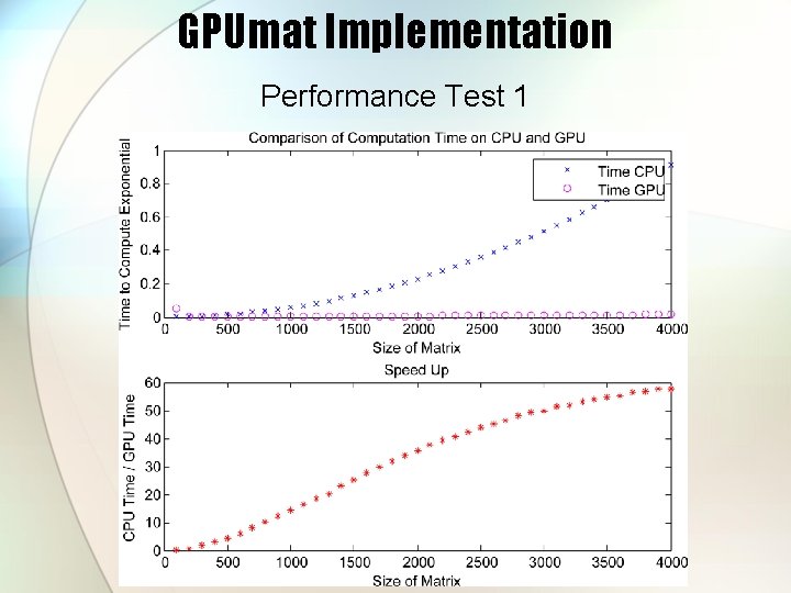
GPUmat Implementation Performance Test 1

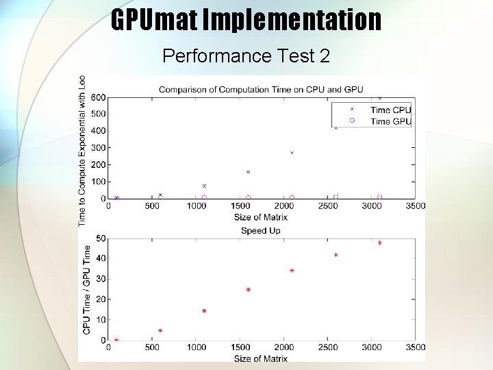
GPUmat Implementation Performance Test 2

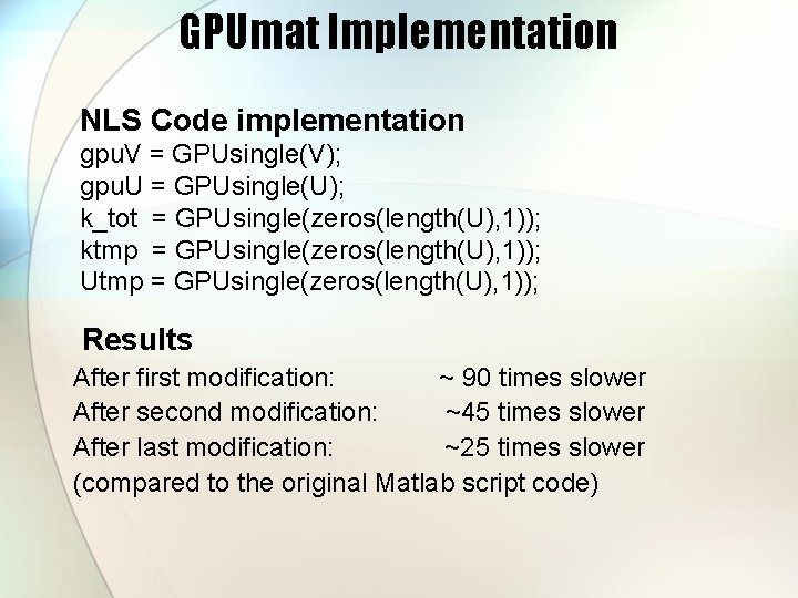
GPUmat Implementation NLS Code implementation gpu. V = GPUsingle(V); gpu. U = GPUsingle(U); k_tot = GPUsingle(zeros(length(U), 1)); ktmp = GPUsingle(zeros(length(U), 1)); Utmp = GPUsingle(zeros(length(U), 1)); Results After first modification: ~ 90 times slower After second modification: ~45 times slower After last modification: ~25 times slower (compared to the original Matlab script code)

GPUmat Implementation Disadvantages: At the beginning of this project • Matlab built-in function ‘sum’ has a bug : had to make a loop for a sum of a matrix • Vert cat error : had to change all arrays in hor cat • Sub-index has to be GPU variable if array is GPU variable : changed vectors to GPU variables • Scalar has to be Matlab variable : changes all GPU variables back to Matlab variables • Matlb built-in functions max/min not included in GPUmat: had to use low level functions cublas. Isamax and cublas. Isamin

GPUmat Implementation Disadvantages: Current Updates • Bugs on ‘sum’ function has been fixed • Vert cat error has been fixed • Sub-index has to be Matlab variable even if array is GPU variable • Scalar has to be Matlab variable : this one stays… • Matlb built-in functions max/min not included in GPUmat: had to use low level functions cublas. Isamax and cublas. Isamin : at least they’re working on it…

GPUmat Implementation Good News: They have completed testing double precision on Windows OS… Currently, they are working on testing double precision on Linux OS… A new project mat. CUDA has been created in sourceforge. net

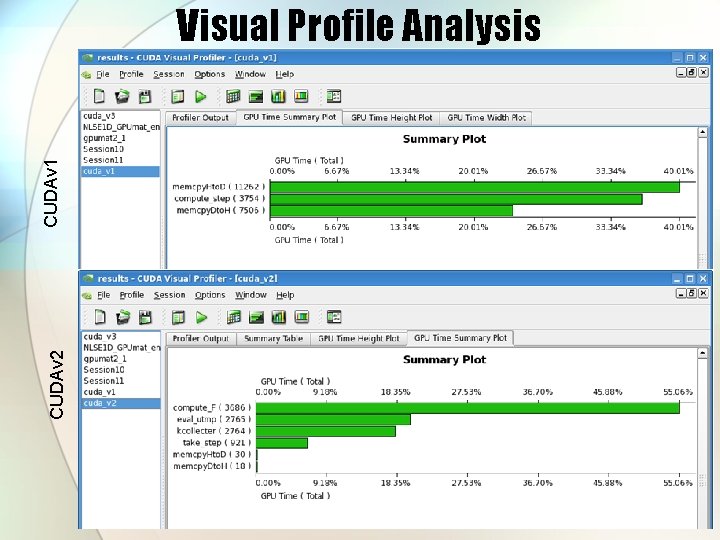
CUDAv 2 CUDAv 1 Visual Profile Analysis

CUDAv 3 GPUmat Visual Profile Analysis

Conclusions Setup of CUDA and MATLAB can be difficult – avoided using our manuals Custom MEX file approach works well Very important to limit memory transfers and to use shared memory GPUmat easy to install and use, but little speedup results for our problem – under development. Final Conclusion: CUDA is worth the development time in order to speed up codes Future work: 2 D and 3 D implementations Other schemes