Simulating a coin toss experiment using Mathematica Kanwaljeet

Simulating a coin toss experiment using Mathematica Kanwaljeet Singh Channey

Consider a virtual experiment of tossing a coin 5 times • Objectives: • Getting the experimental frequency distribution using random numbers • Studying theoretical probability distribution • Comparing theory versus experiment: chisquare minimization

Random Chices • Random. Choice[{a, b, c}, n] • This command randomly selects n objects from the list {a, b, c}. For every new run of the command, we will get a different result just like a true random experiment….

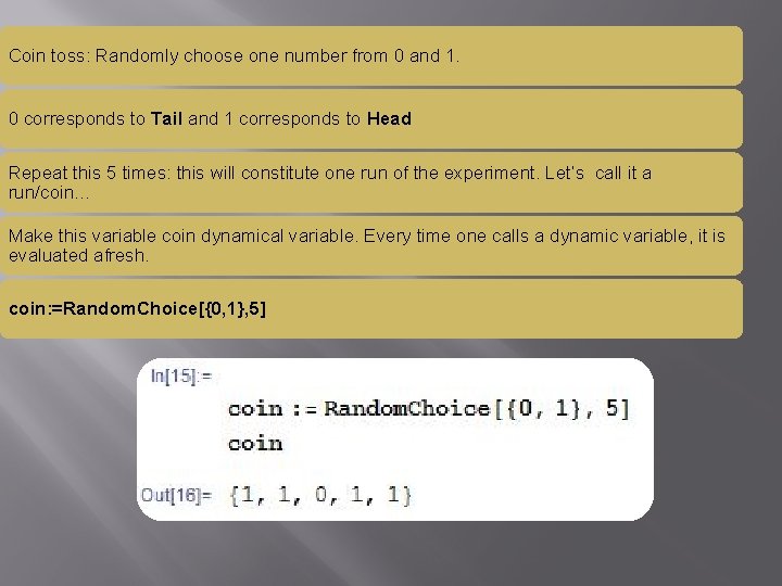
Coin toss: Randomly choose one number from 0 and 1. 0 corresponds to Tail and 1 corresponds to Head Repeat this 5 times: this will constitute one run of the experiment. Let’s call it a run/coin… Make this variable coin dynamical variable. Every time one calls a dynamic variable, it is evaluated afresh. coin: =Random. Choice[{0, 1}, 5]

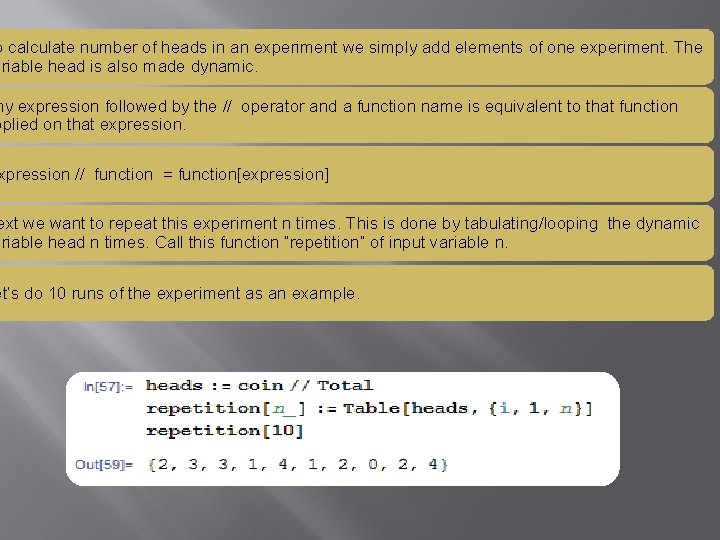
o calculate number of heads in an experiment we simply add elements of one experiment. The ariable head is also made dynamic. ny expression followed by the // operator and a function name is equivalent to that function pplied on that expression. xpression // function = function[expression] ext we want to repeat this experiment n times. This is done by tabulating/looping the dynamic ariable head n times. Call this function “repetition“ of input variable n. et’s do 10 runs of the experiment as an example.

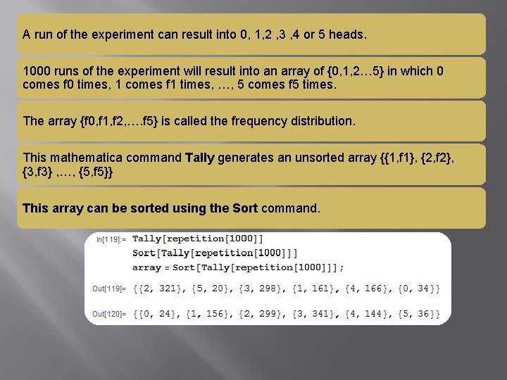
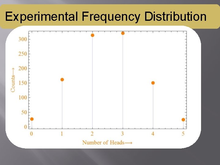
A run of the experiment can result into 0, 1, 2 , 3 , 4 or 5 heads. 1000 runs of the experiment will result into an array of {0, 1, 2… 5} in which 0 comes f 0 times, 1 comes f 1 times, …, 5 comes f 5 times. The array {f 0, f 1, f 2, …. f 5} is called the frequency distribution. This mathematica command Tally generates an unsorted array {{1, f 1}, {2, f 2}, {3, f 3} , …, {5, f 5}} This array can be sorted using the Sort command.

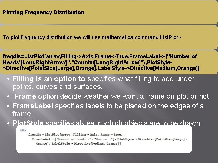
Plotting Frequency Distribution To plot frequency distribution we will use mathematica command List. Plot: freqdis=List. Plot[array, Filling->Axis, Frame->True, Frame. Label->{"Number of Heads[Long. Right. Arrow]", "Counts[Long. Right. Arrow]"}, Plot. Style>Directive[Point. Size[Large], Orange], Label. Style->Directive[Medium, Orange]] • Filling is an option to specifies what filling to add under points, curves and surfaces. • Frame option decide weather we want a frame on plot or not. • Frame. Label specifies labels to be placed on the edges of a frame. • Plot. Style specifies styles in which objects are to be drawn.

Experimental Frequency Distribution

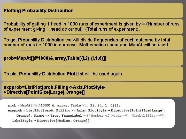
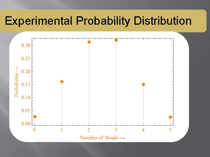
Plotting Probability Distribution Probability of getting 1 head in 1000 runs of experiment is given by = (Number of runs of experiment giving 1 head as output)÷(Total runs of experiment). To get Probability Distribution we will divide frequencies of each outcome by total number of runs i. e 1000 in our case. Mathematica command Map. At will be used prob=Map. At[(#/1000)&, array, Table[{i, 2}, {i, 1, 6}]] To plot Probability Distribution Plot. List will be used again expprob=List. Plot[prob, Filling->Axis, Plot. Style>Directive[Point. Size[Large], Orange]]

Experimental Probability Distribution

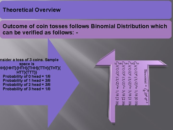
Theoretical Overview Outcome of coin tosses follows Binomial Distribution which can be verified as follows: - onsider a toss of 3 coins. Sample space is HH}{HHT}{HTH}{THH}{TTH}{THT}{ HTT}{TTT}} Probability of 0 head = 1/8 Probability of 1 head = 3/8 Probability of 2 head = 3/8 Probability of 3 head = 1/8

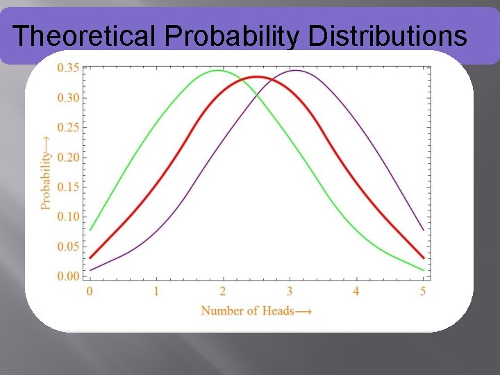
For Binomial Distribution we will be using following mathematica commands Binomial. Distribution[n, p] • represents a binomial distribution with n trials and success probability p. PDF[Binomial. Distribution[n, p], x] • gives the probability density function for the Binomial distribution evaluated at x. We will plot three graphs corresponding to probabilities 0. 4, 0. 5 and 0. 6. To show these three graphs on a single graph for comparison we will use Mathematica Command Show

Theoretical Probability Distributions

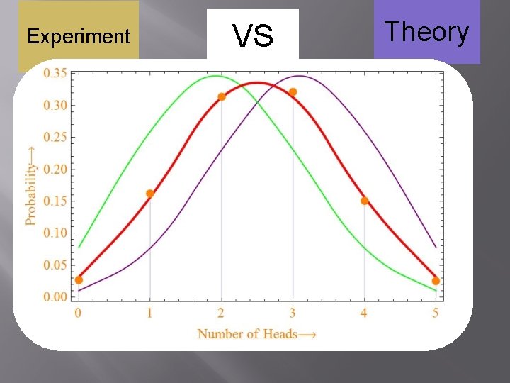
Experiment VS Theory

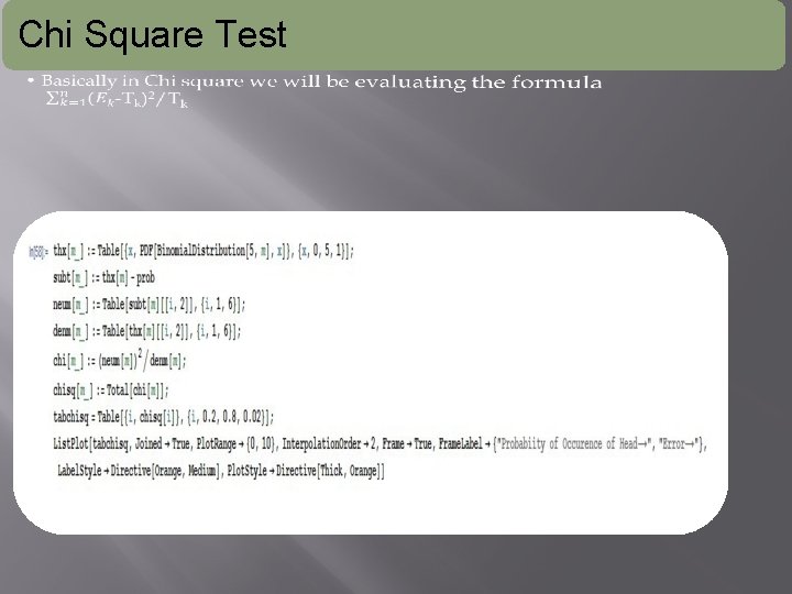
Chi Square Test •

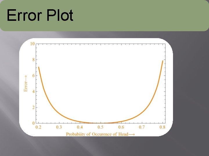
Error Plot

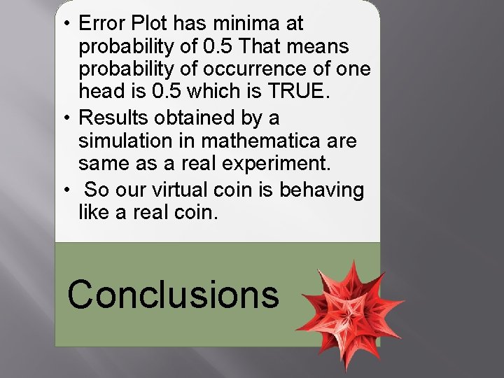
• Error Plot has minima at probability of 0. 5 That means probability of occurrence of one head is 0. 5 which is TRUE. • Results obtained by a simulation in mathematica are same as a real experiment. • So our virtual coin is behaving like a real coin. Conclusions

Thank You.