Simulated Annealing Methods Matthew Kelly April 12 2011

Simulated Annealing Methods Matthew Kelly April 12, 2011

What is Annealing? • Slow cooling of a heated substance allows atoms to line themselves up, creating a stronger structure with minimum energy • Accelerating the cooling process produces a structure with more energy and fewer atoms optimally aligned.

How Does Simulated Annealing Related to Monte Carlo • If system is “cooled quickly”, we produce a local but not global minimum • Allowing system to find minimum takes more time but will result in global minimum, i. e. structure with minimum energy • Can be used to solve Travelling Salesman problem, which is NP-Hard – Has many local minima

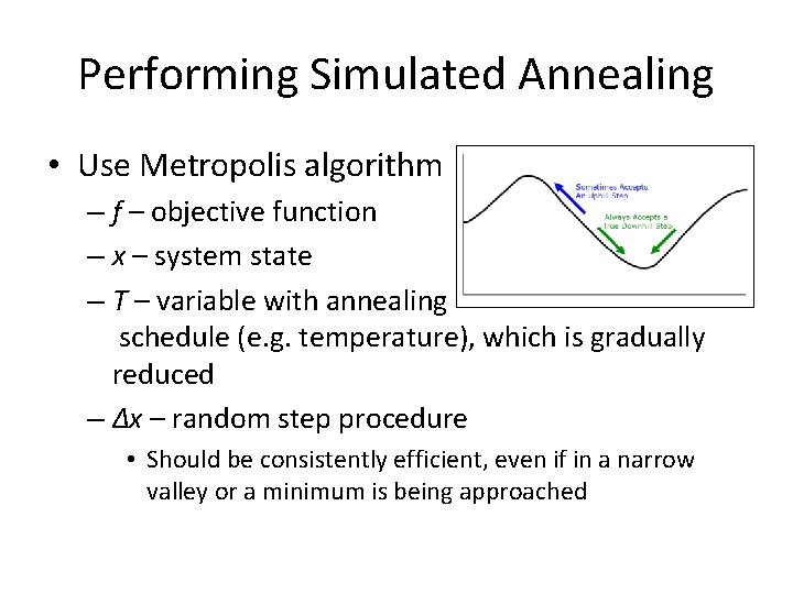
Performing Simulated Annealing • Use Metropolis algorithm – f – objective function – x – system state – T – variable with annealing schedule (e. g. temperature), which is gradually reduced – ∆x – random step procedure • Should be consistently efficient, even if in a narrow valley or a minimum is being approached

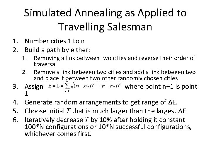
Simulated Annealing as Applied to Travelling Salesman 1. Number cities 1 to n 2. Build a path by either: 1. 2. Removing a link between two cities and reverse their order of traversal Remove a link between two cities and add a link between two and place it between two other randomly chosen cities 3. Assign where point n+1 is point 1 4. Generate random arrangements to get range of ΔE. 5. Choose initial T that is much larger than the largest ΔE. 6. Iteratively decrease T by 10% after holding it constant 100*N configurations or 10*N successful configurations, whichever comes first.

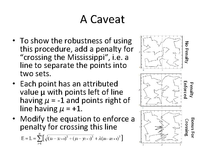
A Caveat No Penalty Enforced Bonus For Crossing • To show the robustness of using this procedure, add a penalty for “crossing the Mississippi”, i. e. a line to separate the points into two sets. • Each point has an attributed value μ with points left of line having μ = -1 and points right of line having μ = +1. • Modify the equation to enforce a penalty for crossing this line

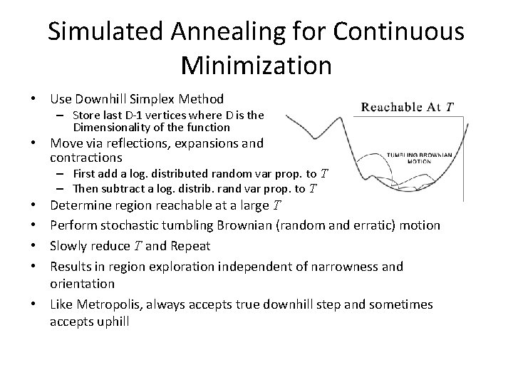
Simulated Annealing for Continuous Minimization • Use Downhill Simplex Method – Store last D-1 vertices where D is the Dimensionality of the function • Move via reflections, expansions and contractions – First add a log. distributed random var prop. to T – Then subtract a log. distrib. rand var prop. to T Determine region reachable at a large T Perform stochastic tumbling Brownian (random and erratic) motion Slowly reduce T and Repeat Results in region exploration independent of narrowness and orientation • Like Metropolis, always accepts true downhill step and sometimes accepts uphill • •

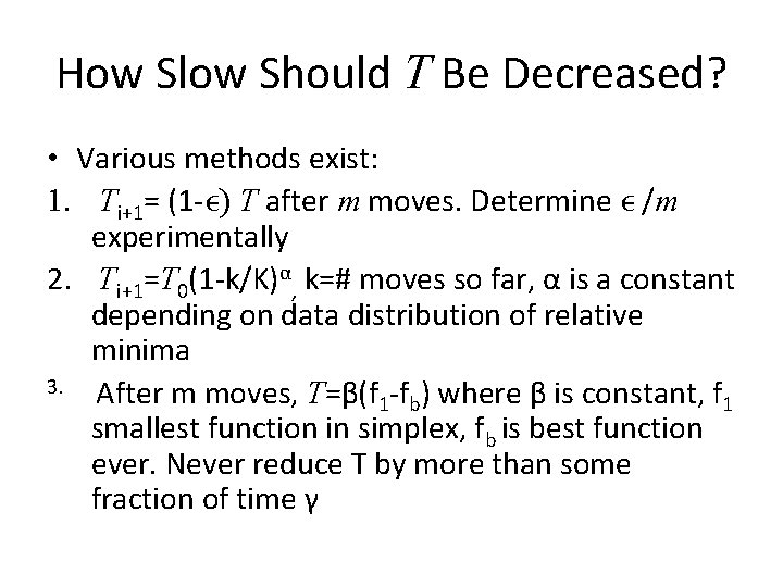
How Slow Should T Be Decreased? • Various methods exist: 1. Ti+1= (1 -ϵ) T after m moves. Determine ϵ /m experimentally 2. Ti+1=T 0(1 -k/K)α, k=# moves so far, α is a constant depending on data distribution of relative minima 3. After m moves, T=β(f -f ) where β is constant, f 1 b 1 smallest function in simplex, fb is best function ever. Never reduce T by more than some fraction of time γ

Advantages of this Method • Not easily fooled by a quick payoff from falling into an unfavorable local minima • Changes that cause large energy differences are sifted over when T is large. – e. g. In travelling salesman, river is cross minimum number of times (2) when T is large due to the large cost (λ) with neglect to correctness of the paths over the weight but are again considered when T is reduced. • Well-correlated with thermodynamics, so has practical use.

Disadvantages of this Method • Degree to which T should be reduced is not clearly defined, 3 potential method are given, all of which don’t work 100% of time • Claim of “effectively solving the traveling salesman problem” does not change the fact that it is an NP problem that would take a long time to resolve. Removing the time characteristic from the method makes attribution to NP (solvable in nondeterministic polynomial time) meaningless. • Scheme of restarting back to a best ever point appears to violate the Metropolis trait of always being able to reach the global minimum regardless of the starting point.