Simplex Method LECTURE 14 MINIMIZATION TWO PHASE METHOD

Simplex Method LECTURE 14 MINIMIZATION TWO PHASE METHOD BY DR. ARSHAD ZAHEER

Two Phase Method

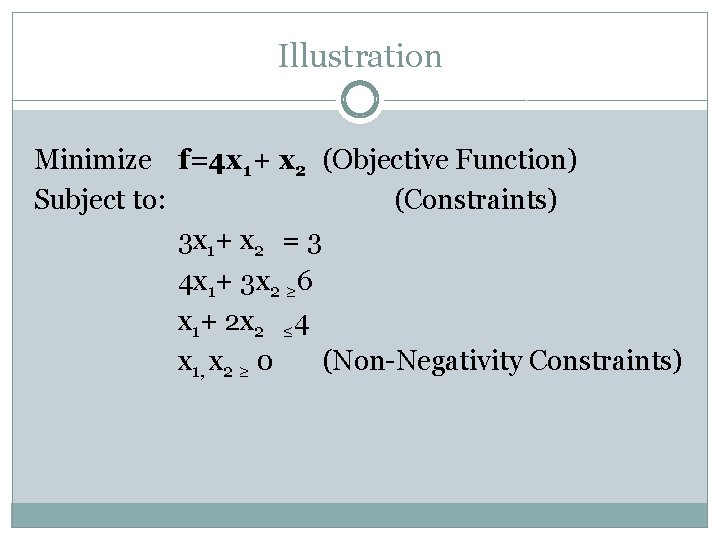
Illustration Minimize f=4 x 1+ x 2 (Objective Function) Subject to: (Constraints) 3 x 1+ x 2 = 3 4 x 1+ 3 x 2 ≥ 6 x 1+ 2 x 2 ≤ 4 x 1, x 2 ≥ 0 (Non-Negativity Constraints)

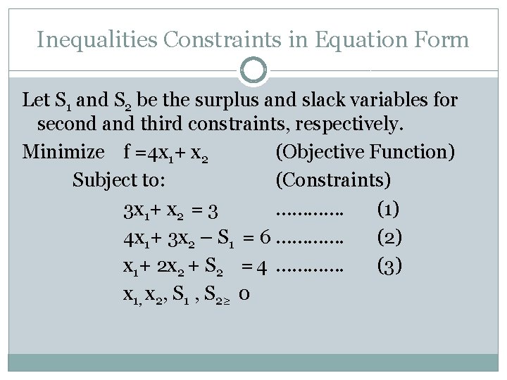
Inequalities Constraints in Equation Form Let S 1 and S 2 be the surplus and slack variables for second and third constraints, respectively. Minimize f =4 x 1+ x 2 (Objective Function) Subject to: (Constraints) 3 x 1+ x 2 = 3 …………. (1) 4 x 1+ 3 x 2 – S 1 = 6 …………. (2) x 1+ 2 x 2 + S 2 = 4 …………. (3) x 1, x 2, S 1 , S 2≥ 0

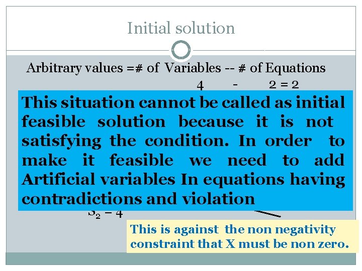
Initial solution Arbitrary values =# of Variables -- # of Equations 4 2=2 Let x 1= 0, x 2 = 0 cannot be called as initial This situation This is against the basic rules of Putting above values in objective function feasible solution because is be not Mathematics as the 0 it cannot (f =5 x 1+ 4 x 2) and equation 1 -3, equal to 3. satisfying the condition. In order to f=0 make it feasible we need to add 0 = 3 (Contradiction) Artificial variables In equations having S 1 = -6 (Violation) contradictions and violation S 2 = 4 This is against the non negativity constraint that X must be non zero.

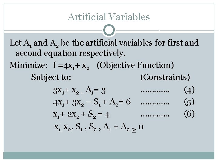
Artificial Variables Let A 1 and A 2 be the artificial variables for first and second equation respectively. Minimize: f =4 x 1+ x 2 (Objective Function) Subject to: (Constraints) 3 x 1+ x 2 + A 1= 3 …………. (4) 4 x 1+ 3 x 2 – S 1 + A 2= 6 …………. (5) x 1+ 2 x 2 + S 2 = 4 …………. (6) x 1, x 2, S 1 , S 2 , A 1 + A 2 ≥ 0

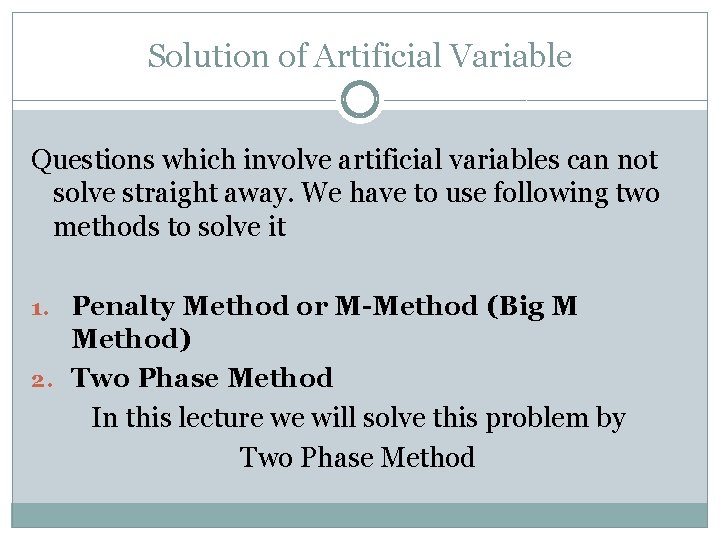
Solution of Artificial Variable Questions which involve artificial variables can not solve straight away. We have to use following two methods to solve it 1. Penalty Method or M-Method (Big M Method) 2. Two Phase Method In this lecture we will solve this problem by Two Phase Method

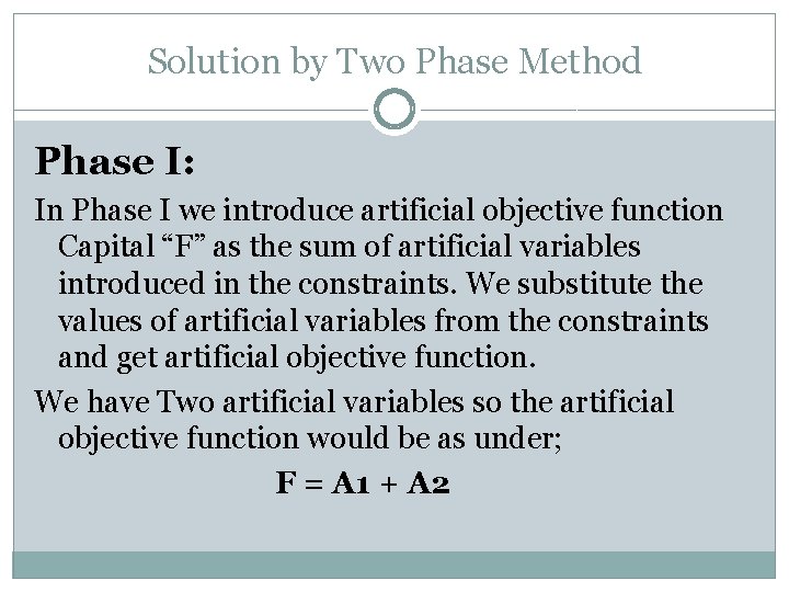
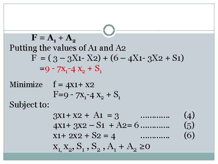
Solution by Two Phase Method Phase I: In Phase I we introduce artificial objective function Capital “F” as the sum of artificial variables introduced in the constraints. We substitute the values of artificial variables from the constraints and get artificial objective function. We have Two artificial variables so the artificial objective function would be as under; F = A 1 + A 2

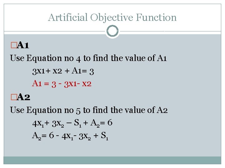
Artificial Objective Function �A 1 Use Equation no 4 to find the value of A 1 3 x 1+ x 2 + A 1= 3 A 1 = 3 - 3 x 1 - x 2 �A 2 Use Equation no 5 to find the value of A 2 4 x 1+ 3 x 2 – S 1 + A 2= 6 - 4 x 1 - 3 x 2 + S 1

F = A 1 + A 2 Putting the values of A 1 and A 2 F = ( 3 – 3 X 1 - X 2) + (6 – 4 X 1 - 3 X 2 + S 1) =9 - 7 x 1 -4 x 2 + S 1 Minimize Subject to: f = 4 x 1+ x 2 F=9 - 7 x 1 -4 x 2 + S 1 3 x 1+ x 2 + A 1 = 3 …………. 4 x 1+ 3 x 2 – S 1 + A 2= 6 …………. x 1+ 2 x 2 + S 2 = 4 …………. x 1, x 2, S 1 , S 2 , A 1 + A 2 ≥ 0 (4) (5) (6)

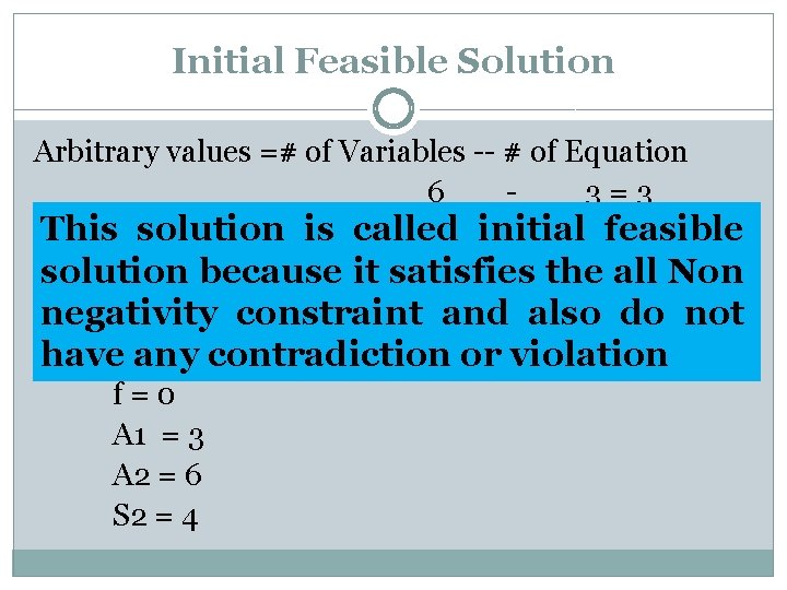
Initial Feasible Solution Arbitrary values =# of Variables -- # of Equation 6 3=3 This solution is =called initial feasible Let x 1= 0, x 2 = 0, S 1 0 solution because itobjective satisfies the all Non Putting above values in functions and equation constraint 4 -6, negativity and also do not = 9 contradiction or violation have. F any f=0 A 1 = 3 A 2 = 6 S 2 = 4

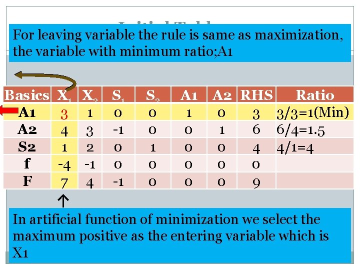
Initial Tableau For leaving variable the rule is same as maximization, the variable with minimum ratio; A 1 Basics A 1 A 2 S 2 f F X 1 3 4 1 -4 7 X 2 S 1 1 0 3 -1 2 0 -1 0 4 -1 S 2 0 0 1 0 0 A 1 1 0 0 A 2 RHS Ratio 0 3 3/3=1(Min) 1 6 6/4=1. 5 0 4 4/1=4 0 0 0 9 ↑ In artificial function of minimization we select the maximum positive as the entering variable which is X 1

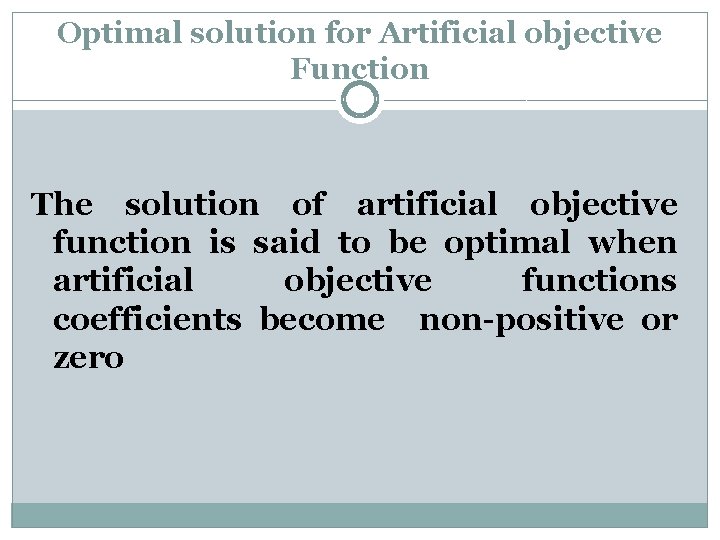
Optimal solution for Artificial objective Function The solution of artificial objective function is said to be optimal when artificial objective functions coefficients become non-positive or zero

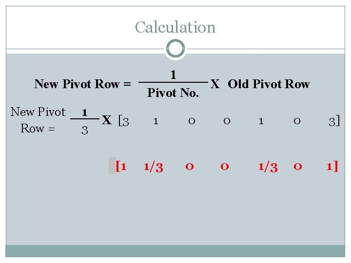
Calculation New Pivot Row = 1 3 X [3 [1 1 X Old Pivot Row Pivot No. 1 0 0 1 0 3] 1/3 0 0 1/3 0 1]

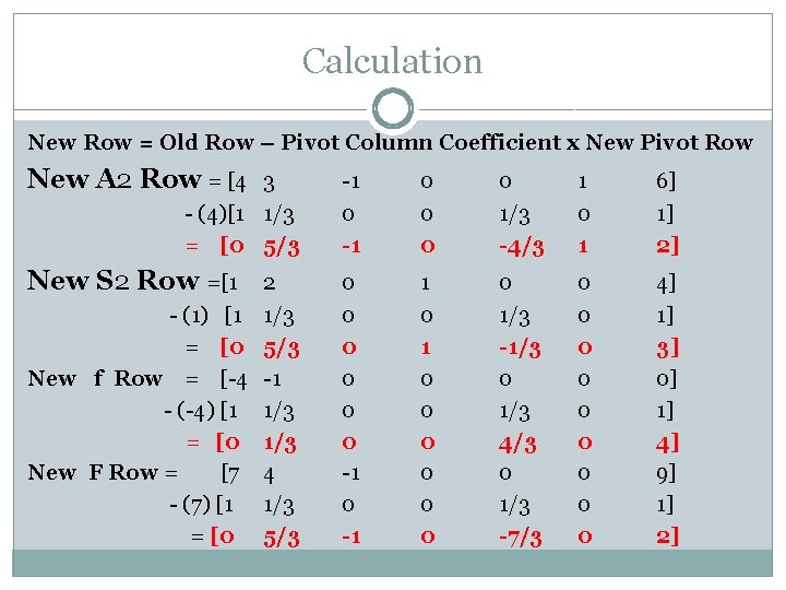
Calculation New Row = Old Row – Pivot Column Coefficient x New Pivot Row New A 2 Row = [4 -1 0 0 0 0 1/3 -4/3 1 0 1 6] 1] 2] New S 2 Row =[1 0 0 0 -1 1 0 0 0 0 1/3 -1/3 0 1/3 4/3 0 1/3 -7/3 0 0 0 0 0 4] 1] 3] 0] 1] 4] 9] 1] 2] 3 - (4)[1 1/3 = [0 5/3 2 - (1) [1 1/3 = [0 5/3 New f Row = [-4 -1 - (-4) [1 1/3 = [0 1/3 New F Row = [7 4 - (7) [1 1/3 = [0 5/3

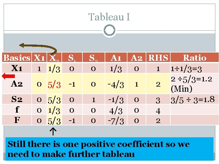
Tableau I Basics X 1 X 2 S 1 X 1 1 1/3 0 S 2 0 A 1 1/3 A 2 0 5/3 -1 0 -4/3 S 2 f F 0 5/3 0 0 1/3 0 0 5/3 -1 1 0 0 -1/3 4/3 -7/3 ↑ A 2 RHS Ratio 0 1 1÷ 1/3=3 2 ÷ 5/3=1. 2 1 2 (Min) 0 3 3/5 ÷ 3=1. 8 0 4 0 2 Still there is one positive coefficient so we need to make further tableau

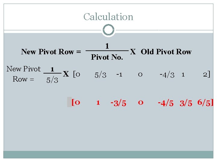
Calculation New Pivot Row = New Pivot 1 X [0 5/3 Row = [0 1 X Old Pivot Row Pivot No. 5/3 -1 0 -4/3 1 2] 1 -3/5 0 -4/5 3/5 6/5]

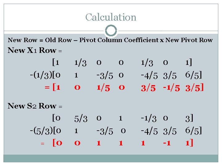
Calculation New Row = Old Row – Pivot Column Coefficient x New Pivot Row New X 1 Row = [1 -(1/3)[0 = [1 1/3 1 0 0 0 -3/5 0 1/3 0 1] -4/5 3/5 6/5] 3/5 -1/5 3/5] 5/3 1 0 0 1 -3/5 0 1 1 -1/3 0 -4/5 3/5 1 -1 New S 2 Row = [0 -(5/3)[0 = [0 3] 6/5] 1]

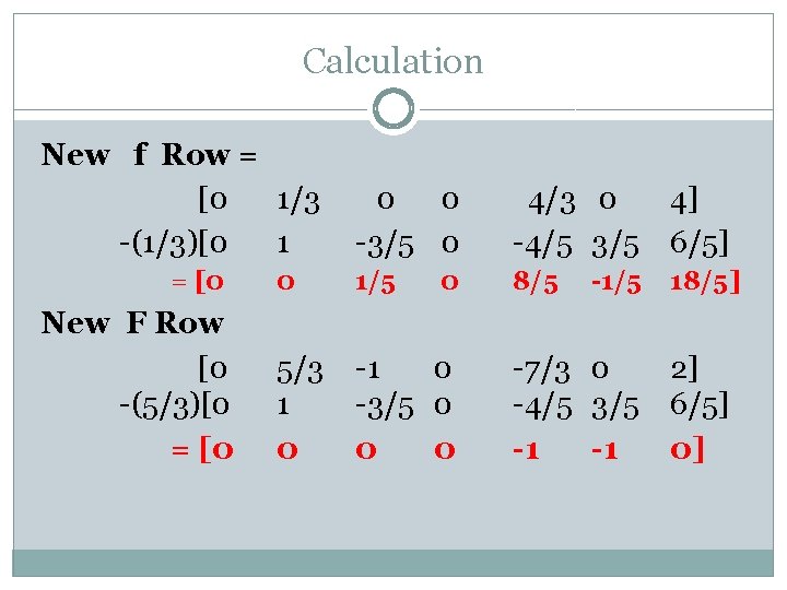
Calculation New f Row = [0 1/3 -(1/3)[0 1 = [0 New F Row [0 -(5/3)[0 = [0 0 0 -3/5 0 4/3 0 -4/5 3/5 4] 6/5] 0 1/5 8/5 18/5] 5/3 1 0 -3/5 0 0 -1/5 -7/3 0 -4/5 3/5 -1 -1 2] 6/5] 0]

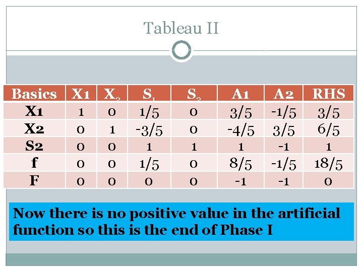
Tableau II Basics X 1 X 2 S 2 f F X 1 X 2 1 0 0 0 0 S 1 1/5 -3/5 1 1/5 0 S 2 0 0 1 0 0 A 1 3/5 -4/5 1 8/5 -1 A 2 -1/5 3/5 -1 -1/5 -1 RHS 3/5 6/5 1 18/5 0 Now there is no positive value in the artificial function so this is the end of Phase I

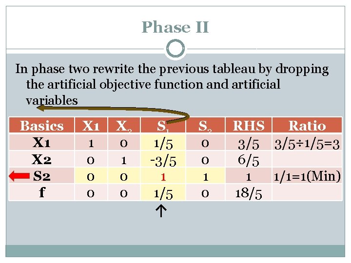
Phase II In phase two rewrite the previous tableau by dropping the artificial objective function and artificial variables Basics X 1 X 2 S 2 f X 1 1 0 0 0 X 2 0 1 0 0 S 1 1/5 -3/5 1 1/5 ↑ S 2 0 0 1 0 RHS Ratio 3/5÷ 1/5=3 6/5 1 1/1=1(Min) 18/5

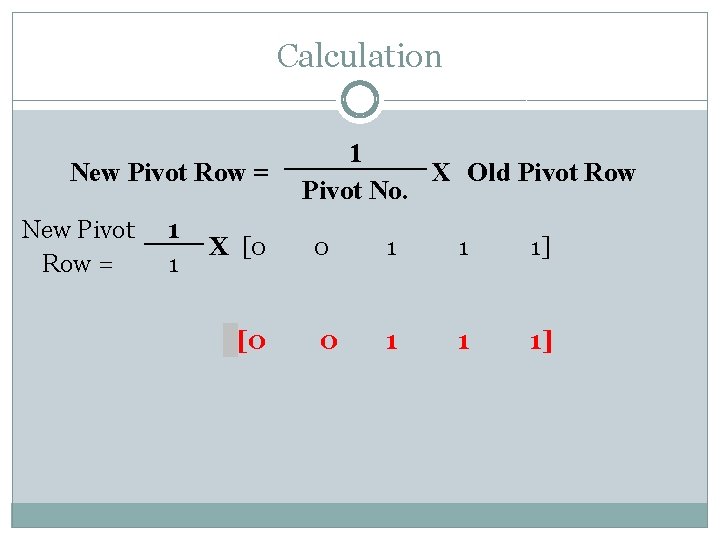
Calculation New Pivot Row = 1 1 X [0 [0 1 X Old Pivot Row Pivot No. 0 1 1 1]

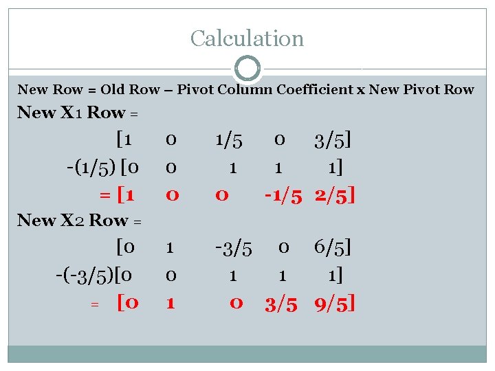
Calculation New Row = Old Row – Pivot Column Coefficient x New Pivot Row New X 1 Row = [1 -(1/5) [0 = [1 0 0 0 1/5 1 0 0 3/5] 1 1] -1/5 2/5] 1 0 1 -3/5 0 6/5] 1 1 1] 0 3/5 9/5] New X 2 Row = [0 -(-3/5)[0 = [0

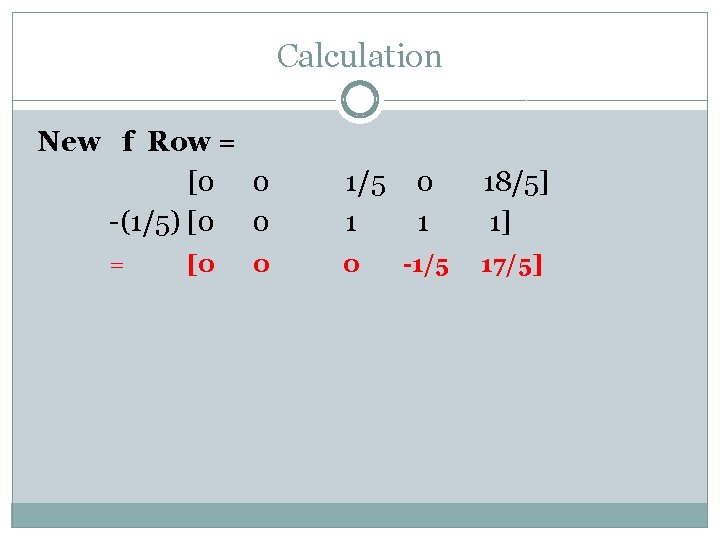
Calculation New f Row = [0 0 -(1/5) [0 0 = [0 0 1/5 1 0 0 1 18/5] 1] -1/5 17/5]

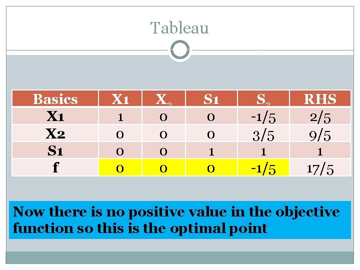
Tableau Basics X 1 X 2 S 1 f X 1 1 0 0 0 X 2 0 0 S 1 0 0 1 0 S 2 -1/5 3/5 1 -1/5 RHS 2/5 9/5 1 17/5 Now there is no positive value in the objective function so this is the optimal point

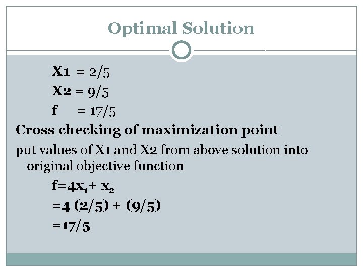
Optimal Solution X 1 = 2/5 X 2 = 9/5 f = 17/5 Cross checking of maximization point put values of X 1 and X 2 from above solution into original objective function f=4 x 1+ x 2 =4 (2/5) + (9/5) =17/5

Thank You