Simplex Method Continued from a presentation at the

Simplex Method Continued … from a presentation at the Fuqua School of Business MIT and James Orlin © 2003 Rev. 2. 71 by M. Miccio on December 15, 2014 file Simplex 2_AMII_05 b_gr MIT and James Orlin © 2003 1

Today’s Lecture l l l Review of the simplex algorithm Alternative Optimal Solutions Unbounded Solution Degeneracy Is the simplex algorithm finite? (Answer, yes, but only if we are careful) MIT and James Orlin © 2003 2

Today’s Lecture l l l Review of the simplex algorithm Alternative Optimal Solutions Unbounded Solution Degeneracy Is the simplex algorithm finite? (Answer, yes, but only if we are careful) MIT and James Orlin © 2003 3

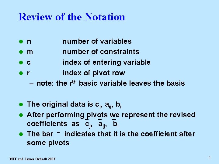
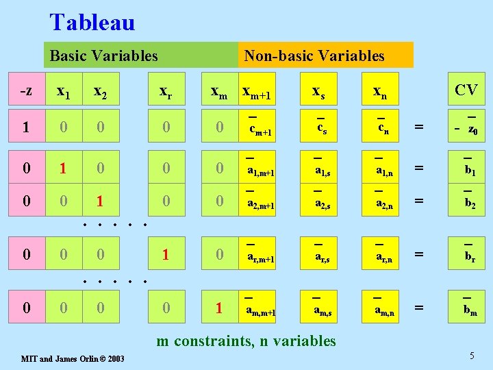
Review of the Notation n number of variables l m number of constraints l c index of entering variable l r index of pivot row – note: the rth basic variable leaves the basis l The original data is cj, aij, bi l After performing pivots we represent the revised coefficients as cj, aij, bi l The bar − indicates that it is the coefficient after some pivots l MIT and James Orlin © 2003 4

Tableau Basic Variables Non-basic Variables -z x 1 x 2 xr xm xm+1 xs xn 1 0 0 cm+1 cs cn = - z 0 0 1 0 0 0 a 1, m+1 a 1, s a 1, n = b 1 0 0 a 2, m+1 a 2, s a 2, n = b 2 0 0 0 1 0 ar, m+1 ar, s ar, n = br 0 0 1 am, m+1 am, s am, n = bm . . CV m constraints, n variables MIT and James Orlin © 2003 5

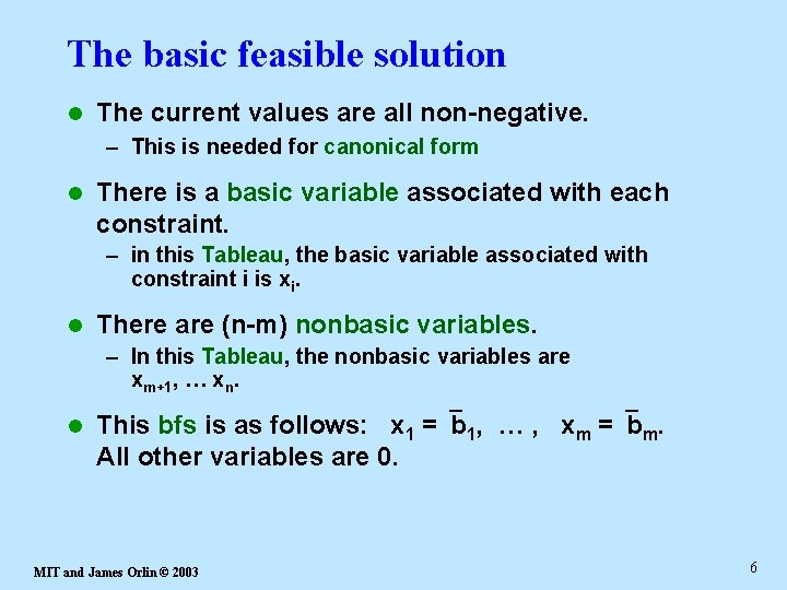
The basic feasible solution l The current values are all non-negative. – This is needed for canonical form l There is a basic variable associated with each constraint. – in this Tableau, the basic variable associated with constraint i is xi. l There are (n-m) nonbasic variables. – In this Tableau, the nonbasic variables are xm+1, … xn. l This bfs is as follows: x 1 = b 1, … , xm = bm. All other variables are 0. MIT and James Orlin © 2003 6

Today’s Lecture l l l Review of the simplex algorithm. Alternative Optimal Solutions Unbounded Solution Degeneracy Degenerate Solutions Proving finiteness and optimality under no degeneracy MIT and James Orlin © 2003 7

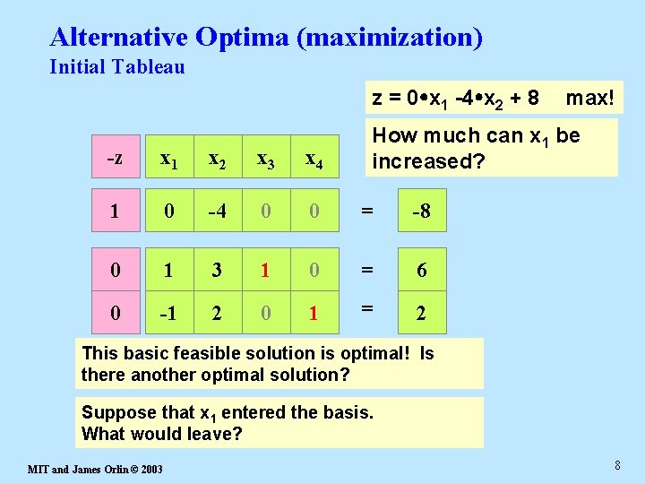
Alternative Optima (maximization) Initial Tableau z = 0 x 1 -4 x 2 + 8 max! How much can x 1 be increased? -z x 1 x 2 x 3 x 4 1 0 -4 0 0 = -8 0 1 3 1 0 = 6 0 -1 2 0 1 = 2 This basic feasible solution is optimal! Is there another optimal solution? Suppose that x 1 entered the basis. What would leave? MIT and James Orlin © 2003 8

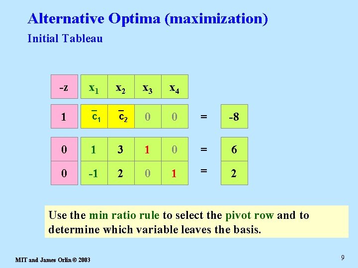
Alternative Optima (maximization) Initial Tableau -z x 1 x 2 x 3 x 4 1 c 01 c -42 0 0 = -8 0 1 3 1 0 = 6 0 -1 2 0 1 = 2 Use the min ratio rule to select the pivot row and to determine which variable leaves the basis. MIT and James Orlin © 2003 9

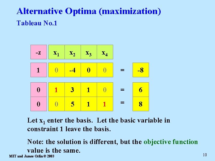
Alternative Optima (maximization) Tableau No. 1 -z x 1 x 2 x 3 x 4 1 0 -4 0 0 = -8 0 1 3 1 0 = 6 0 -1 0 52 10 1 = 82 Let x 1 enter the basis. Let the basic variable in constraint 1 leave the basis. Note: the solution is different, but the objective function value is the same. MIT and James Orlin © 2003 10

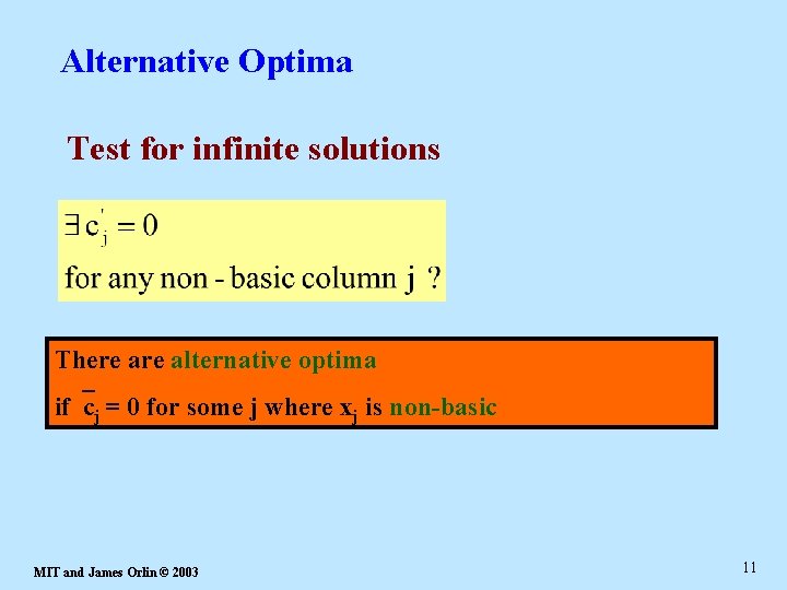
Alternative Optima Test for infinite solutions There alternative optima if cj = 0 for some j where xj is non-basic MIT and James Orlin © 2003 11

Today’s Lecture l l l Review of the simplex algorithm. Alternative Optimal Solutions Unbounded Solution Degeneracy Degenerate Solutions Proving finiteness and optimality under no degeneracy MIT and James Orlin © 2003 12

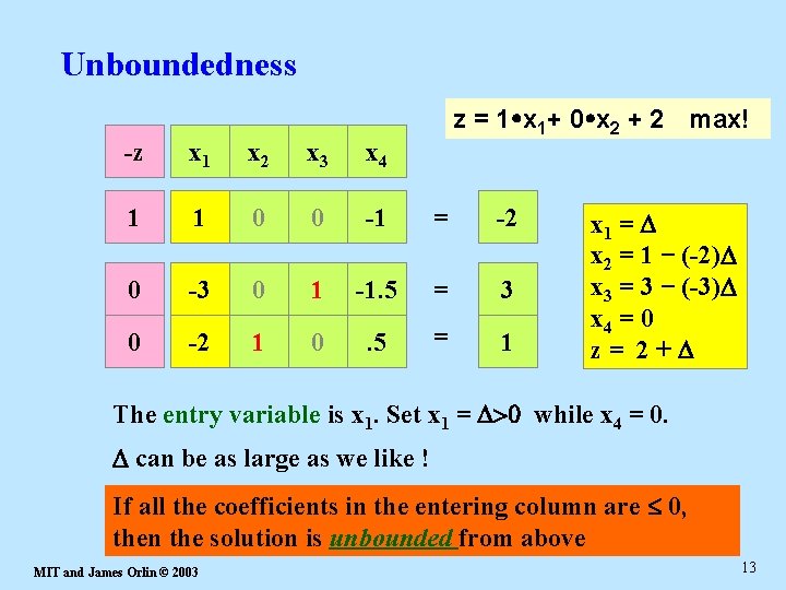
Unboundedness z = 1 x 1+ 0 x 2 + 2 max! -z x 1 x 2 x 3 x 4 1 1 0 0 -1 = -2 0 -3 0 1 -1. 5 = 3 0 -2 1 0 . 5 = 1 x 1 = D = 0 x 2 = 1 − (-2)D = 1 x 3 = 3 − (-3)D = 3 x 4 = 0 z = 2 + D The entry variable is x 1. Set x 1 = D>0 while x 4 = 0. D can be as large as we like ! If all the coefficients in the entering column are 0, then the solution is unbounded from above MIT and James Orlin © 2003 13

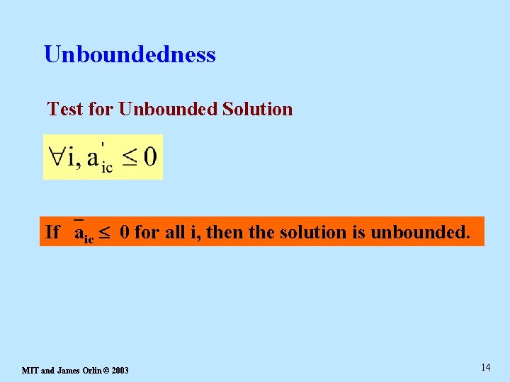
Unboundedness Test for Unbounded Solution If aic 0 for all i, then the solution is unbounded. MIT and James Orlin © 2003 14

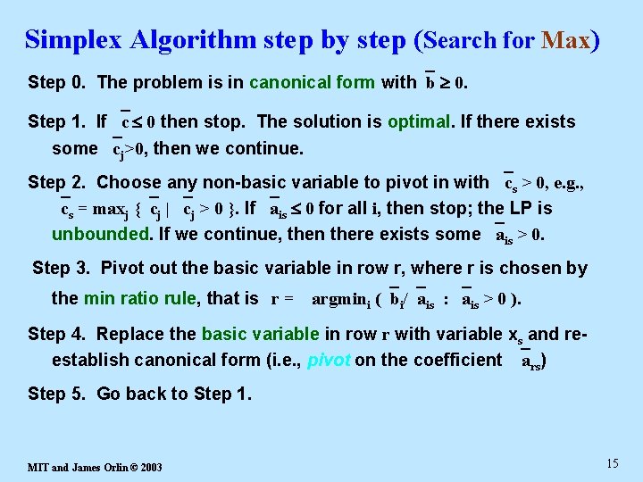
Simplex Algorithm step by step (Search for Max) Step 0. The problem is in canonical form with b 0. Step 1. If c 0 then stop. The solution is optimal. If there exists some cj>0, then we continue. Step 2. Choose any non-basic variable to pivot in with cs > 0, e. g. , cs = maxj { cj | cj > 0 }. If ais 0 for all i, then stop; the LP is unbounded. If we continue, then there exists some ais > 0. Step 3. Pivot out the basic variable in row r, where r is chosen by the min ratio rule, that is r = argmini ( bi/ ais : ais > 0 ). Step 4. Replace the basic variable in row r with variable xs and reestablish canonical form (i. e. , pivot on the coefficient ars) Step 5. Go back to Step 1. MIT and James Orlin © 2003 15

Today’s Lecture l l l Review of the simplex algorithm. Alternative Optimal Solutions Unbounded Solution Degeneracy and Degenerate Solutions Proving finiteness and optimality under no degeneracy MIT and James Orlin © 2003 16

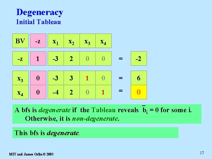
Degeneracy Initial Tableau BV -z x 1 x 2 x 3 x 4 -z 1 -3 2 0 0 = -2 x 3 0 -3 3 1 0 = 6 x 4 0 -4 2 0 1 = 02 A bfs is degenerate if the Tableau reveals bi = 0 for some i. Otherwise, it is non-degenerate. This bfs is degenerate. MIT and James Orlin © 2003 17

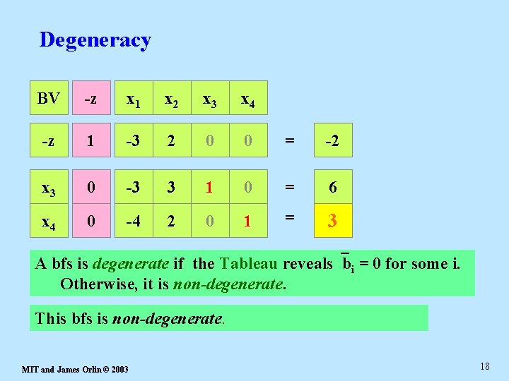
Degeneracy BV -z x 1 x 2 x 3 x 4 -z 1 -3 2 0 0 = -2 x 3 0 -3 3 1 0 = 6 x 4 0 -4 2 0 1 = 32 A bfs is degenerate if the Tableau reveals bi = 0 for some i. Otherwise, it is non-degenerate. This bfs is non-degenerate. MIT and James Orlin © 2003 18

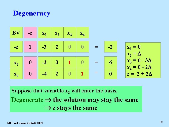
Degeneracy BV -z x 1 x 2 x 3 x 4 -z 1 -3 2 0 0 = -2 x 3 0 -3 3 1 0 = 6 x 4 0 -4 2 0 1 = 02 x 1 = 0 x 2 = D x 3 = 6 - 3 D x 4 = 0 - 2 D z = 2 + 2 D Suppose that variable x 2 will enter the basis. Degenerate the solution may stay the same z stays the same MIT and James Orlin © 2003 19

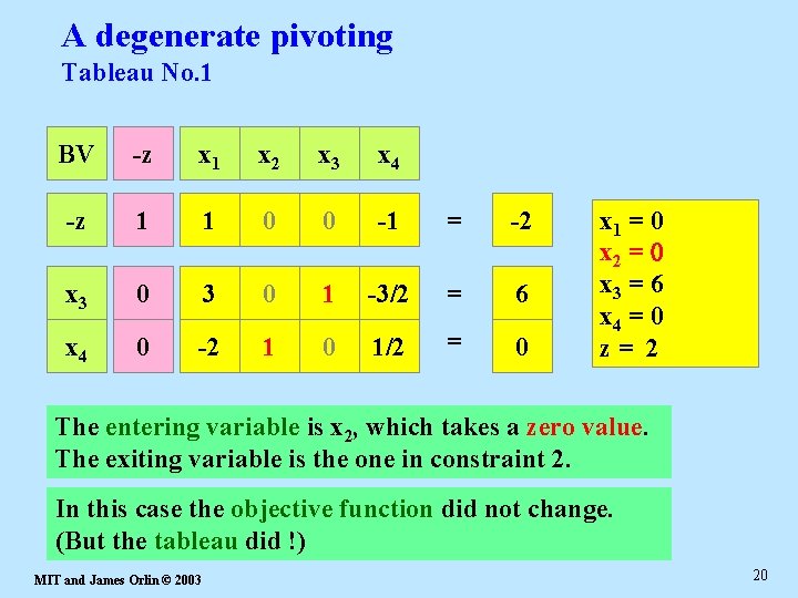
A degenerate pivoting Tableau No. 1 BV -z x 1 x 2 x 3 x 4 -z 1 -3 1 02 0 -1 0 = -2 x 3 0 -3 3 03 1 -3/2 0 = 6 x 4 0 -4 -2 12 0 1/2 1 = 0 x 1 = 0 x 2 = 0 x 3 = 6 x 4 = 0 z = 2 The entering variable is x 2, which takes a zero value. The exiting variable is the one in constraint 2. In this case the objective function did not change. (But the tableau did !) MIT and James Orlin © 2003 20

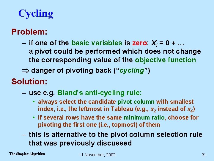
Cycling Problem: – if one of the basic variables is zero: Xi = 0 + … a pivot could be performed which does not change the corresponding value of the objective function danger of pivoting back (“cycling”) Solution: – use e. g. Bland’s anti-cycling rule: • always select the candidate pivot column with smallest index, i. e. , the leftmost in Tableau (e. g. , x 2 instead of x 4) • if several rows have the same minimum ratio, choose for pivoting the first one (i. e. , topmost) of them – this is alternative to the pivot column selection rule that was previously discussed The Simplex Algorithm 11 November, 2002 21

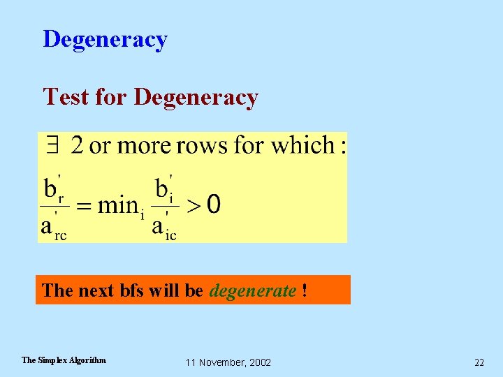
Degeneracy Test for Degeneracy The next bfs will be degenerate ! The Simplex Algorithm 11 November, 2002 22

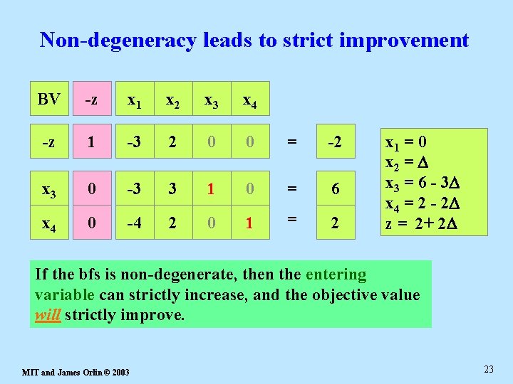
Non-degeneracy leads to strict improvement BV -z x 1 x 2 x 3 x 4 -z 1 -3 2 0 0 = -2 x 3 0 -3 3 1 0 = 6 x 4 0 -4 2 0 1 = 2 x 1 = 0 x 2 = D x 3 = 6 - 3 D x 4 = 2 - 2 D z = 2+ 2 D If the bfs is non-degenerate, then the entering variable can strictly increase, and the objective value will strictly improve. MIT and James Orlin © 2003 23

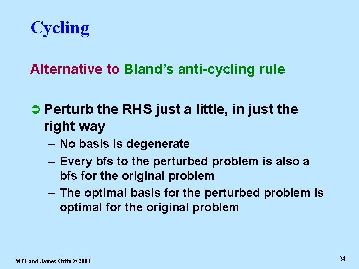
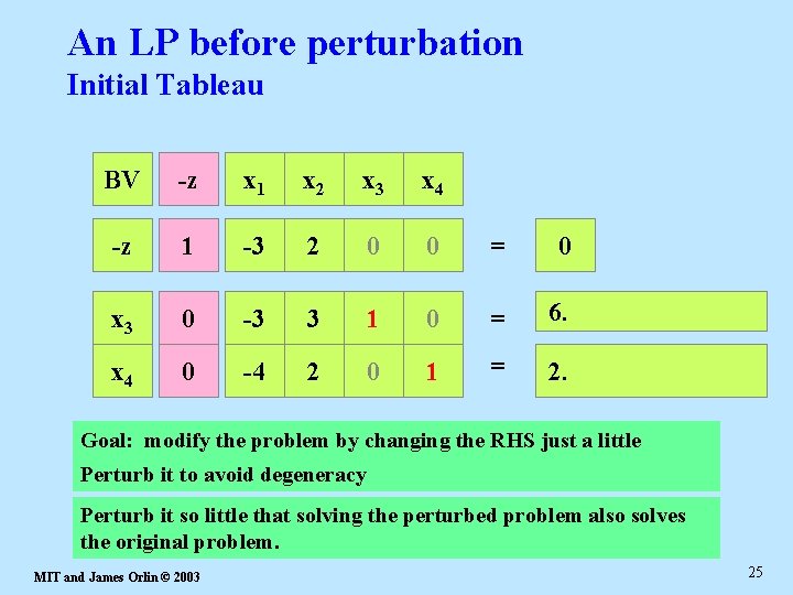
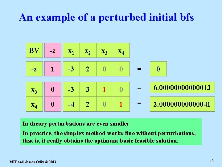
Cycling Alternative to Bland’s anti-cycling rule Perturb the RHS just a little, in just the right way – No basis is degenerate – Every bfs to the perturbed problem is also a bfs for the original problem – The optimal basis for the perturbed problem is optimal for the original problem MIT and James Orlin © 2003 24

An LP before perturbation Initial Tableau BV -z x 1 x 2 x 3 x 4 -z 1 -3 2 0 0 = x 3 0 -3 3 1 0 = 6. x 4 0 -4 2 0 1 = 2. 0 Goal: modify the problem by changing the RHS just a little Perturb it to avoid degeneracy Perturb it so little that solving the perturbed problem also solves the original problem. MIT and James Orlin © 2003 25

An example of a perturbed initial bfs BV -z x 1 x 2 x 3 x 4 -z 1 -3 2 0 0 = x 3 0 -3 3 1 0 = 6. 00000013 x 4 0 -4 2 0 1 = 2. 00000041 0 In theory perturbations are even smaller In practice, the simplex method works fine without perturbations, that is, it really obtains the optimum basic feasible solution. MIT and James Orlin © 2003 26

Today’s Lecture l l l Review of the simplex algorithm. Alternative Optimal Solutions Unbounded Solution Degeneracy Degenerate Solutions Proving finiteness and optimality under no degeneracy MIT and James Orlin © 2003 27

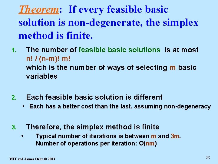
Theorem: If every feasible basic solution is non-degenerate, the simplex method is finite. 1. The number of feasible basic solutions is at most n! / (n-m)! m! which is the number of ways of selecting m basic variables 2. Each feasible basic solution is different • Each has a better cost than the last, assuming non-degeneracy Therefore, the simplex method is finite 3. • Typical number of iterations is between m and 3 m. Number of operations per iteration: O(nm) MIT and James Orlin © 2003 28

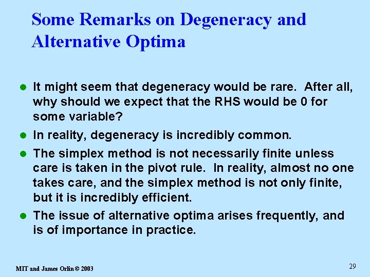
Some Remarks on Degeneracy and Alternative Optima l It might seem that degeneracy would be rare. After all, why should we expect that the RHS would be 0 for some variable? In reality, degeneracy is incredibly common. l The simplex method is not necessarily finite unless care is taken in the pivot rule. In reality, almost no one takes care, and the simplex method is not only finite, but it is incredibly efficient. l The issue of alternative optima arises frequently, and is of importance in practice. l MIT and James Orlin © 2003 29

Software for Simplex implementation and solution

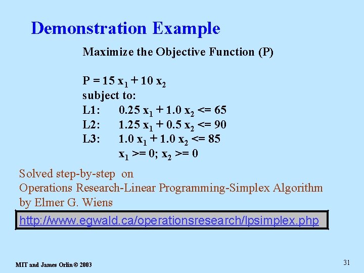
Demonstration Example Maximize the Objective Function (P) P = 15 x 1 + 10 x 2 subject to: L 1: 0. 25 x 1 + 1. 0 x 2 <= 65 L 2: 1. 25 x 1 + 0. 5 x 2 <= 90 L 3: 1. 0 x 1 + 1. 0 x 2 <= 85 x 1 >= 0; x 2 >= 0 Solved step-by-step on Operations Research-Linear Programming-Simplex Algorithm by Elmer G. Wiens http: //www. egwald. ca/operationsresearch/lpsimplex. php MIT and James Orlin © 2003 31

Demonstration Simplex solver Solved step-by-step Tableau and Final Solution on Finite mathematics utility: simplex method tool http: //www. zweigmedia. com/Real. World/simplex. html MIT and James Orlin © 2003 32

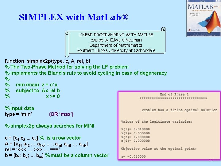
SIMPLEX with Mat. Lab® LINEAR PROGRAMMING WITH MATLAB course by Edward Neuman Department of Mathematics Southern Illinois University at Carbondale function simplex 2 p(type, c, A, rel, b) % The Two-Phase Method for solving the LP problem % implements the Bland’s rule to avoid cycling in case of degeneracy % % min (max) z = c*x % subject to Ax rel b % x >= 0. . . % input data type = ‘min’ (OR ‘max’) % simplex 2 p always searches for MIN! c = [c 1 c 2. . . ck] % is a row vector A = [a 11 a 12 … a 1 k; . . . ; am 1 am 2 … amk] rel = ‘<<< … >>> … ===‘ b = [b 1; b 2; . . . bm] % must be a column vector 33

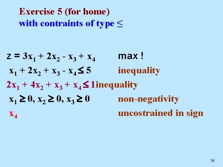
Exercise 5 (for home) with contraints of type ≤ z = 3 x 1 + 2 x 2 - x 3 + x 4 max ! x 1 + 2 x 2 + x 3 - x 4 5 inequality 2 x 1 + 4 x 2 + x 3 + x 4 1 inequality x 1 0, x 2 0, x 3 0 non-negativity x 4 uncostrained in sign 34