Simple Linear Regression Susanta Nag Assistant Professor Department

Simple Linear Regression Susanta Nag Assistant Professor Department of Economics Central University of Jammu

Introduction to Regression Analysis The term regression was coined by Francis Galton Regression shows the casual/functional relationship between variables or shows average relationship between two or more variables. Regression is used to: Estimate or Predict the value of a dependent variable (Y) on the basis of the value of at least one independent variable Explain the impact of changes in an independent variable on the dependent variable Dependent variable: the variable we wish to explain Independent variable: the variable used to explain the dependent variable

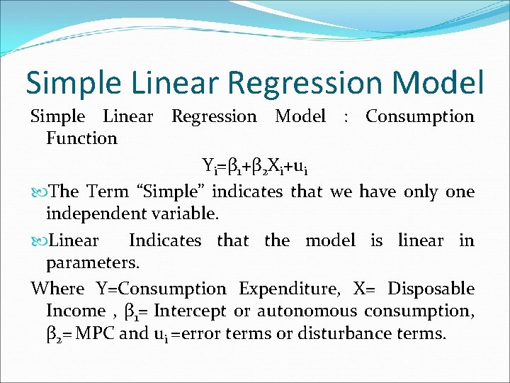
Simple Linear Regression Model : Consumption Function Yi=β 1+β 2 Xi+ui The Term “Simple” indicates that we have only one independent variable. Linear Indicates that the model is linear in parameters. Where Y=Consumption Expenditure, X= Disposable Income , β 1= Intercept or autonomous consumption, β 2= MPC and ui =error terms or disturbance terms.

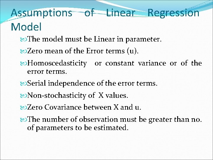
Assumptions Model of Linear Regression The model must be Linear in parameter. Zero mean of the Error terms (u). Homoscedasticity error terms. or constant variance or of the Serial independence of the error terms. Non-stochasticity of X values. Zero Covariance between X and u. The number of observation must be greater than no. of parameters to be estimated.

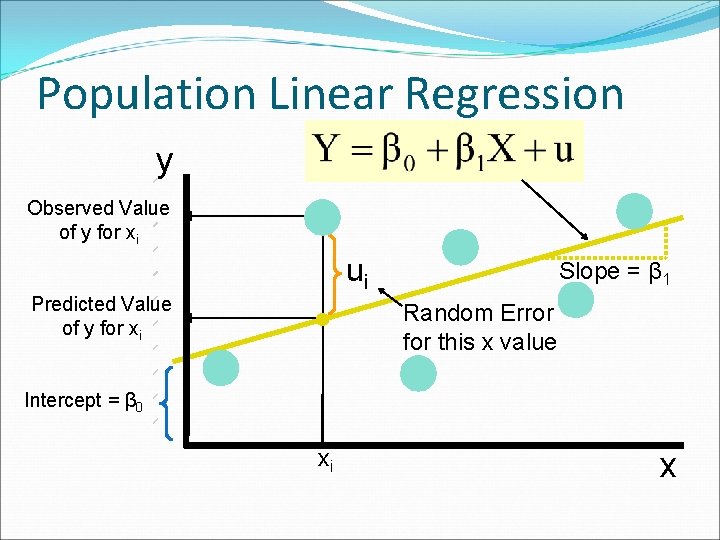
Population Linear Regression y Observed Value of y for xi ui Predicted Value of y for xi Slope = β 1 Random Error for this x value Intercept = β 0 xi x

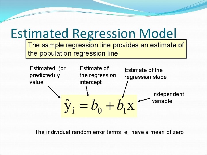
Estimated Regression Model The sample regression line provides an estimate of the population regression line Estimated (or predicted) y value Estimate of the regression intercept Estimate of the regression slope Independent variable The individual random error terms ei have a mean of zero

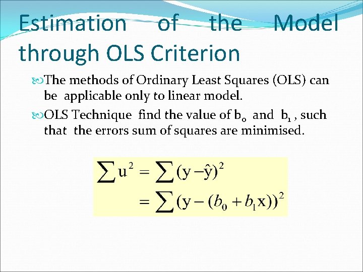
Estimation of the through OLS Criterion Model The methods of Ordinary Least Squares (OLS) can be applicable only to linear model. OLS Technique find the value of b 0 and b 1 , such that the errors sum of squares are minimised.

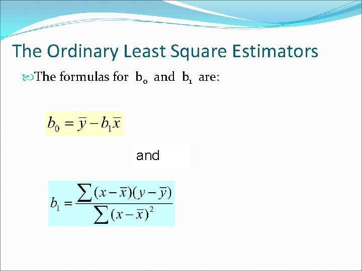
The Ordinary Least Square Estimators The formulas for b 0 and b 1 are: and

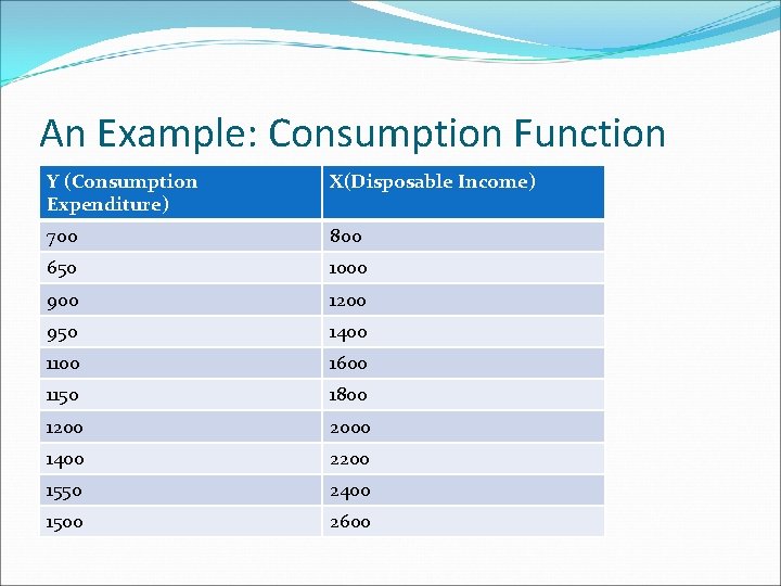
An Example: Consumption Function Y (Consumption Expenditure) X(Disposable Income) 700 800 650 1000 900 1200 950 1400 1100 1600 1150 1800 1200 2000 1400 2200 1550 2400 1500 2600

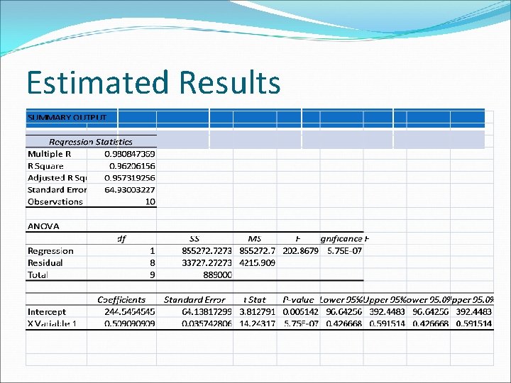
Estimated Results

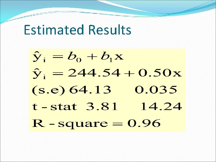
Estimated Results

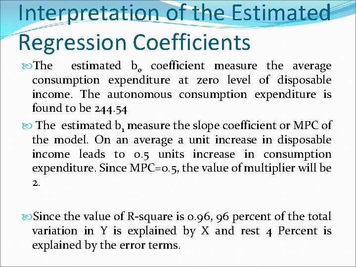
Interpretation of the Estimated Regression Coefficients The estimated b 0 coefficient measure the average consumption expenditure at zero level of disposable income. The autonomous consumption expenditure is found to be 244. 54 The estimated b 1 measure the slope coefficient or MPC of the model. On an average a unit increase in disposable income leads to 0. 5 units increase in consumption expenditure. Since MPC=0. 5, the value of multiplier will be 2. Since the value of R-square is 0. 96, 96 percent of the total variation in Y is explained by X and rest 4 Percent is explained by the error terms.

Reading List: Basic Econometrics by D N Gujurati , D C Porter and Sangeetha Gunasekhar. Theory of Econometrics by A Koutsoyiannis