Simple Linear Regression An Introduction n n Simple
- Slides: 39

Simple Linear Regression An Introduction n n Simple Linear Regression Model Least Squares Method Coefficient of Determination Model Assumptions Testing for Significance © 2007 Thomson South-Western. All Rights Reserved Slide 1

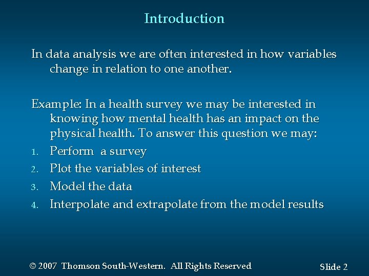
Introduction In data analysis we are often interested in how variables change in relation to one another. Example: In a health survey we may be interested in knowing how mental health has an impact on the physical health. To answer this question we may: 1. Perform a survey 2. Plot the variables of interest 3. Model the data 4. Interpolate and extrapolate from the model results © 2007 Thomson South-Western. All Rights Reserved Slide 2

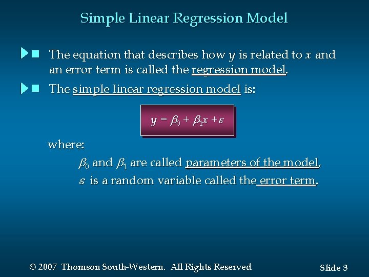
Simple Linear Regression Model n The equation that describes how y is related to x and an error term is called the regression model. n The simple linear regression model is: y = 0 + 1 x + where: 0 and 1 are called parameters of the model, is a random variable called the error term. © 2007 Thomson South-Western. All Rights Reserved Slide 3

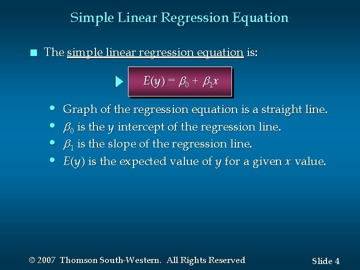
Simple Linear Regression Equation n The simple linear regression equation is: E(y ) = 0 + 1 x • Graph of the regression equation is a straight line. • 0 is the y intercept of the regression line. • 1 is the slope of the regression line. • E(y ) is the expected value of y for a given x value. © 2007 Thomson South-Western. All Rights Reserved Slide 4

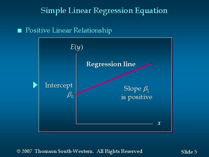
Simple Linear Regression Equation n Positive Linear Relationship E (y ) Regression line Intercept 0 Slope 1 is positive x © 2007 Thomson South-Western. All Rights Reserved Slide 5

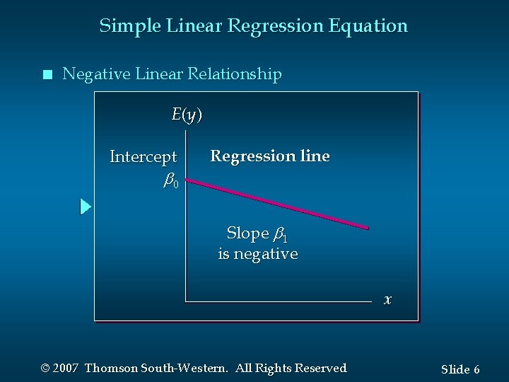
Simple Linear Regression Equation n Negative Linear Relationship E (y ) Intercept 0 Regression line Slope 1 is negative x © 2007 Thomson South-Western. All Rights Reserved Slide 6

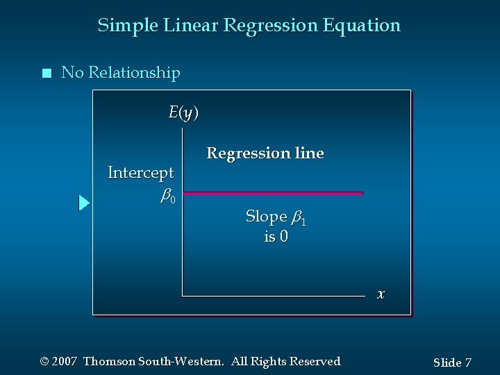
Simple Linear Regression Equation n No Relationship E (y ) Intercept 0 Regression line Slope 1 is 0 x © 2007 Thomson South-Western. All Rights Reserved Slide 7

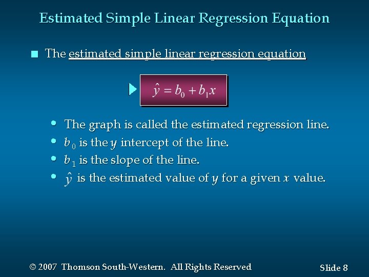
Estimated Simple Linear Regression Equation n The estimated simple linear regression equation • • The graph is called the estimated regression line. b 0 is the y intercept of the line. b 1 is the slope of the line. is the estimated value of y for a given x value. © 2007 Thomson South-Western. All Rights Reserved Slide 8

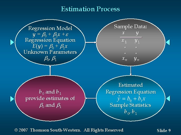
Estimation Process Regression Model y = 0 + 1 x + Regression Equation E ( y ) = 0 + 1 x Unknown Parameters 0, 1 b 0 and b 1 provide estimates of 0 and 1 Sample Data: x y x 1 y 1. . xn y n Estimated Regression Equation Sample Statistics b 0, b 1 © 2007 Thomson South-Western. All Rights Reserved Slide 9

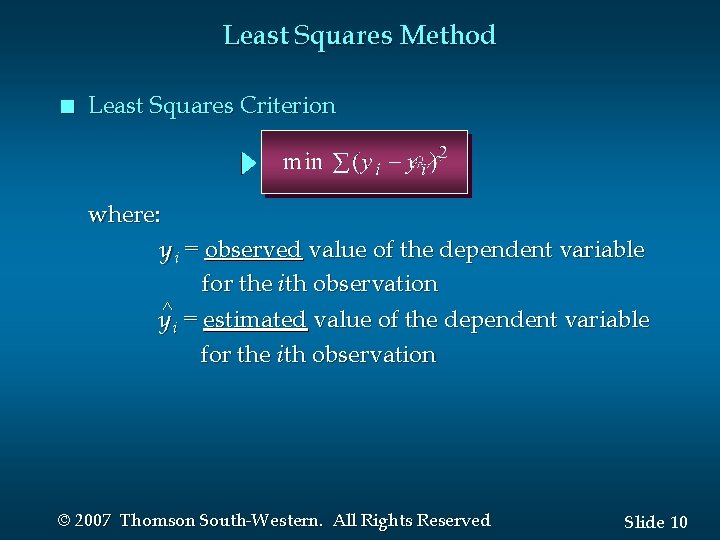
Least Squares Method n Least Squares Criterion where: y i = observed value of the dependent variable for the ith observation y^i = estimated value of the dependent variable for the ith observation © 2007 Thomson South-Western. All Rights Reserved Slide 10

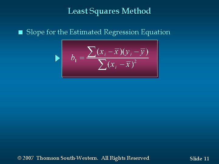
Least Squares Method n Slope for the Estimated Regression Equation © 2007 Thomson South-Western. All Rights Reserved Slide 11

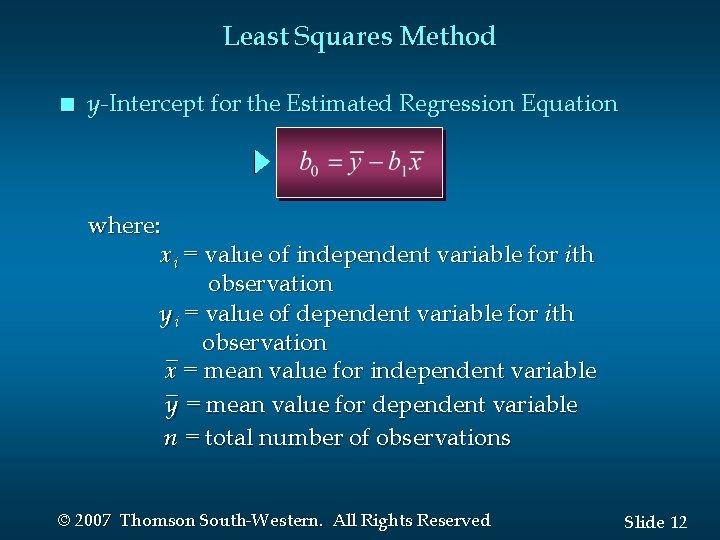
Least Squares Method n y -Intercept for the Estimated Regression Equation where: xi = value of independent variable for ith observation y i = value of dependent variable for ith _ observation x = mean value for independent variable _ y = mean value for dependent variable n = total number of observations © 2007 Thomson South-Western. All Rights Reserved Slide 12

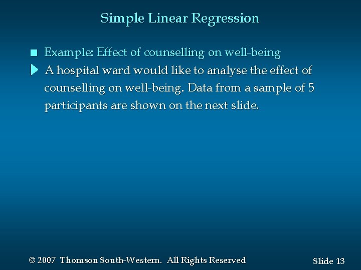
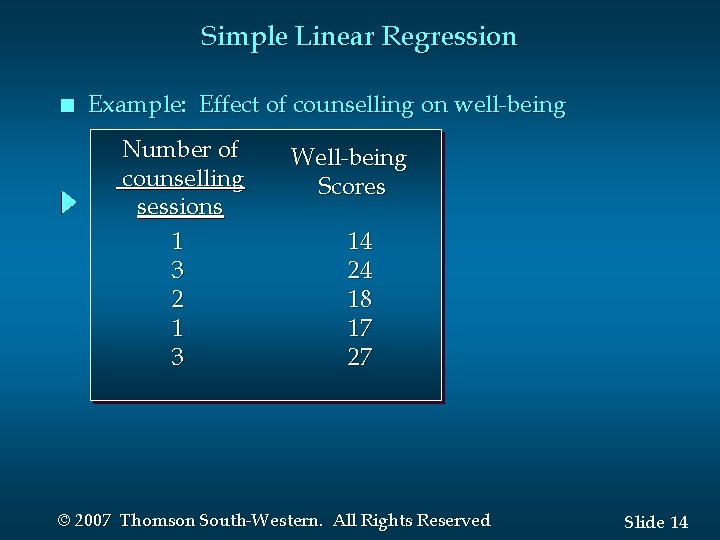
Simple Linear Regression n Example: Effect of counselling on well-being A hospital ward would like to analyse the effect of counselling on well-being. Data from a sample of 5 participants are shown on the next slide. © 2007 Thomson South-Western. All Rights Reserved Slide 13

Simple Linear Regression n Example: Effect of counselling on well-being Number of counselling sessions 1 3 2 1 3 Well-being Scores 14 24 18 17 27 © 2007 Thomson South-Western. All Rights Reserved Slide 14

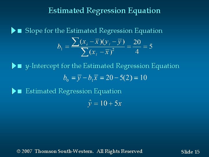
Estimated Regression Equation n Slope for the Estimated Regression Equation n y -Intercept for the Estimated Regression Equation n Estimated Regression Equation © 2007 Thomson South-Western. All Rights Reserved Slide 15

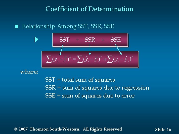
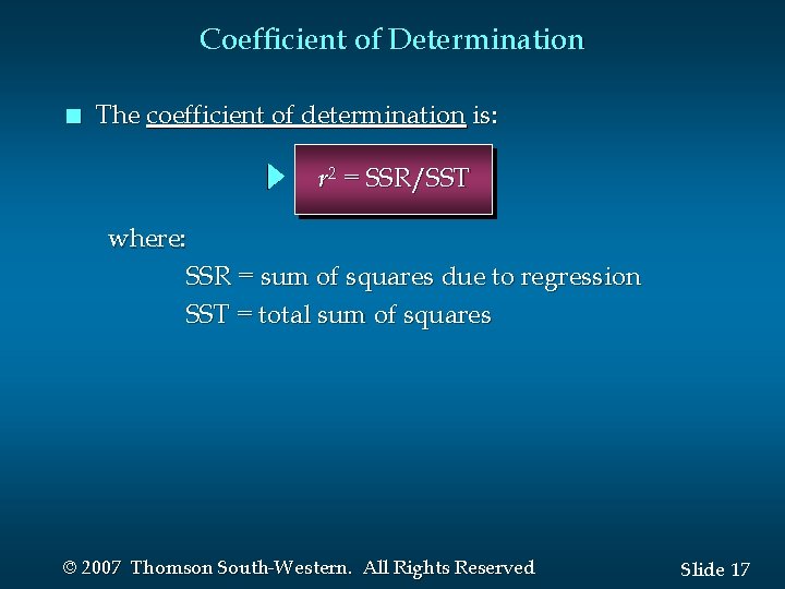
Coefficient of Determination n Relationship Among SST, SSR, SSE SST = SSR + SSE where: SST = total sum of squares SSR = sum of squares due to regression SSE = sum of squares due to error © 2007 Thomson South-Western. All Rights Reserved Slide 16

Coefficient of Determination n The coefficient of determination is: r 2 = SSR/SST where: SSR = sum of squares due to regression SST = total sum of squares © 2007 Thomson South-Western. All Rights Reserved Slide 17

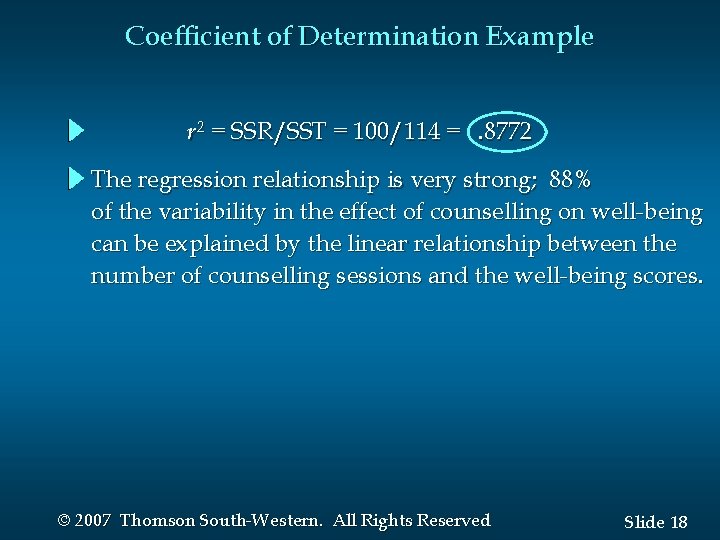
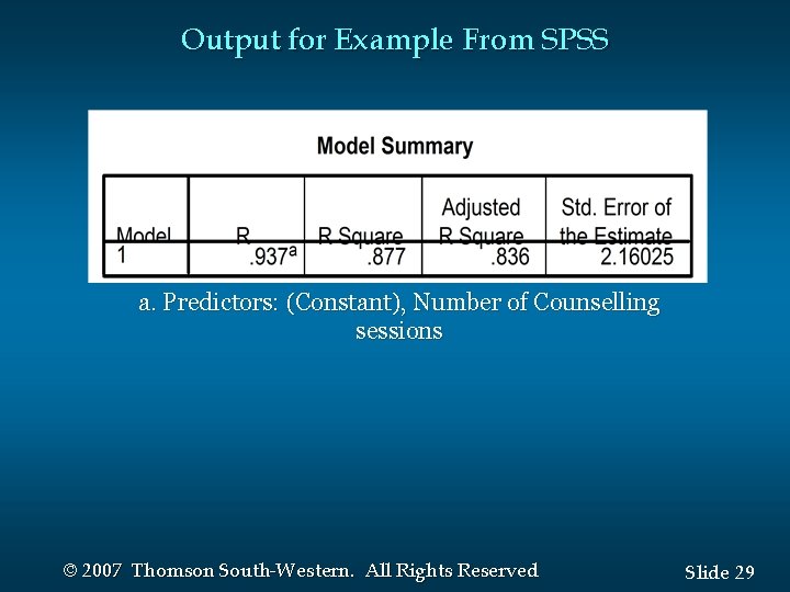
Coefficient of Determination Example r 2 = SSR/SST = 100/114 =. 8772 The regression relationship is very strong; 88% of the variability in the effect of counselling on well-being can be explained by the linear relationship between the number of counselling sessions and the well-being scores. © 2007 Thomson South-Western. All Rights Reserved Slide 18

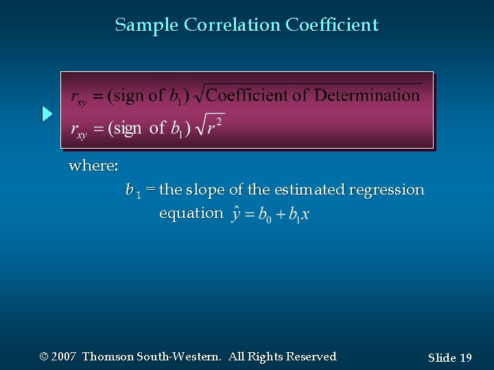
Sample Correlation Coefficient where: b 1 = the slope of the estimated regression equation © 2007 Thomson South-Western. All Rights Reserved Slide 19

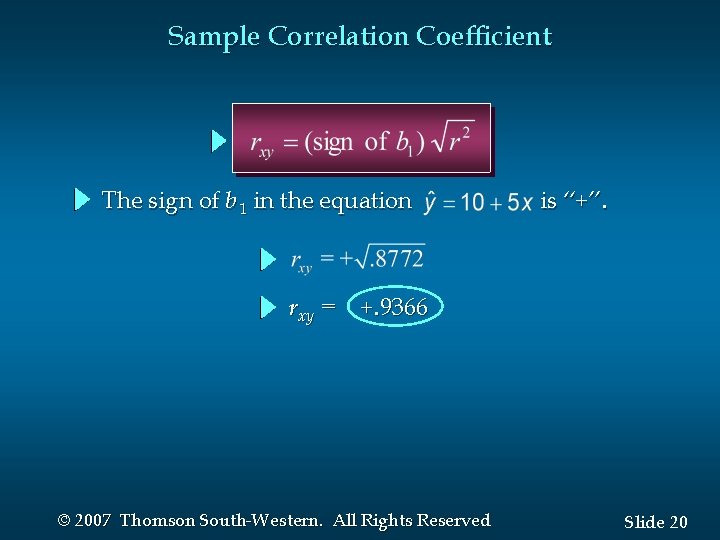
Sample Correlation Coefficient The sign of b 1 in the equation is “+”. rxy = +. 9366 © 2007 Thomson South-Western. All Rights Reserved Slide 20

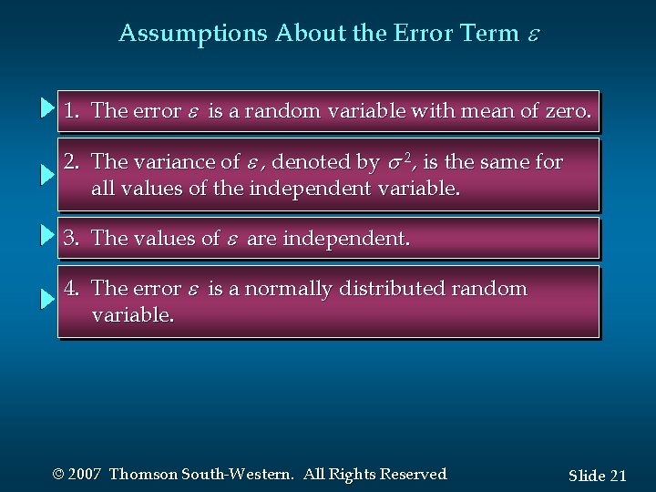
Assumptions About the Error Term 1. The error is a random variable with mean of zero. 2. The variance of , denoted by 2, is the same for all values of the independent variable. 3. The values of are independent. 4. The error is a normally distributed random variable. © 2007 Thomson South-Western. All Rights Reserved Slide 21

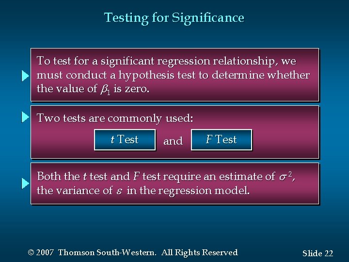
Testing for Significance To test for a significant regression relationship, we must conduct a hypothesis test to determine whether the value of 1 is zero. Two tests are commonly used: t Test and F Test Both the t test and F test require an estimate of 2, the variance of in the regression model. © 2007 Thomson South-Western. All Rights Reserved Slide 22

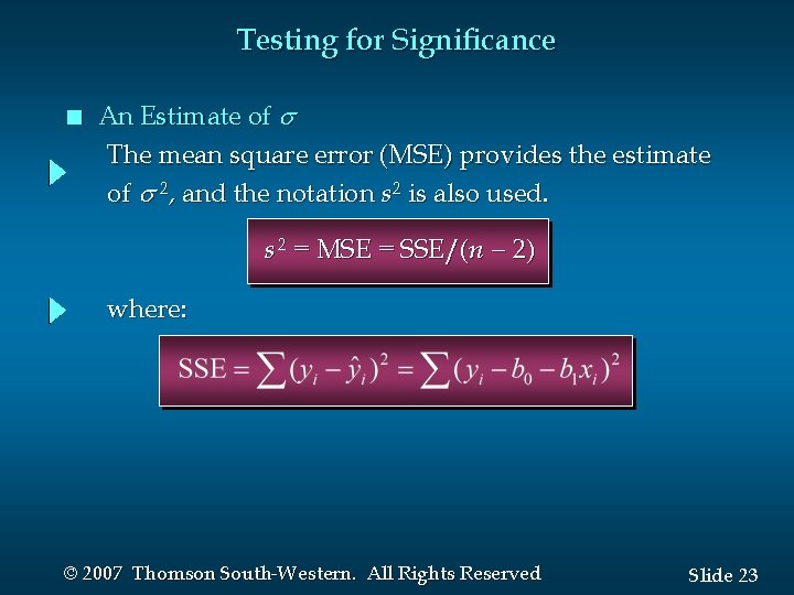
Testing for Significance n An Estimate of The mean square error (MSE) provides the estimate of 2, and the notation s 2 is also used. s 2 = MSE = SSE/(n - 2) where: © 2007 Thomson South-Western. All Rights Reserved Slide 23

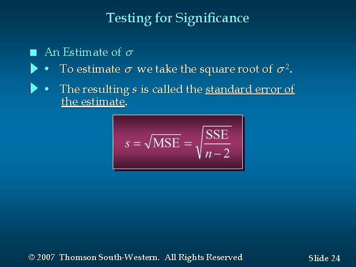
Testing for Significance n An Estimate of • To estimate we take the square root of 2. • The resulting s is called the standard error of the estimate. © 2007 Thomson South-Western. All Rights Reserved Slide 24

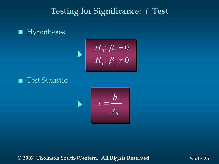
Testing for Significance: t Test n Hypotheses n Test Statistic © 2007 Thomson South-Western. All Rights Reserved Slide 25

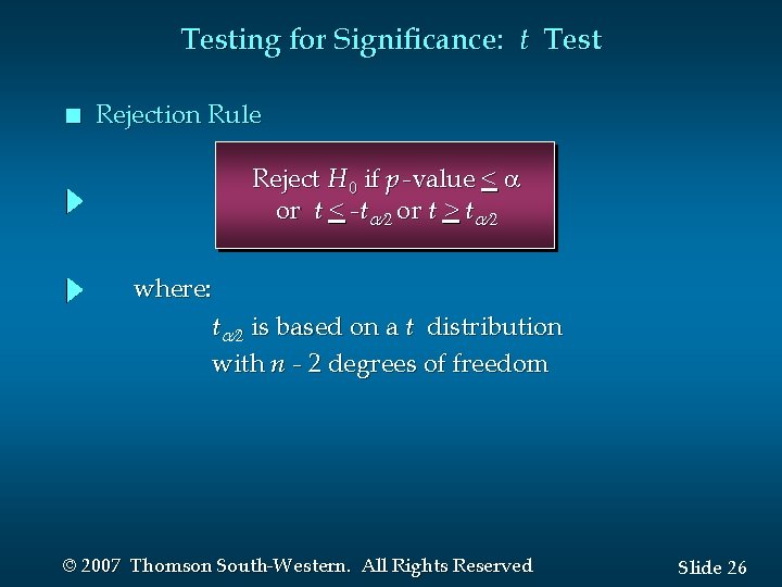
Testing for Significance: t Test n Rejection Rule Reject H 0 if p -value < a or t < -t or t > t where: t is based on a t distribution with n - 2 degrees of freedom © 2007 Thomson South-Western. All Rights Reserved Slide 26

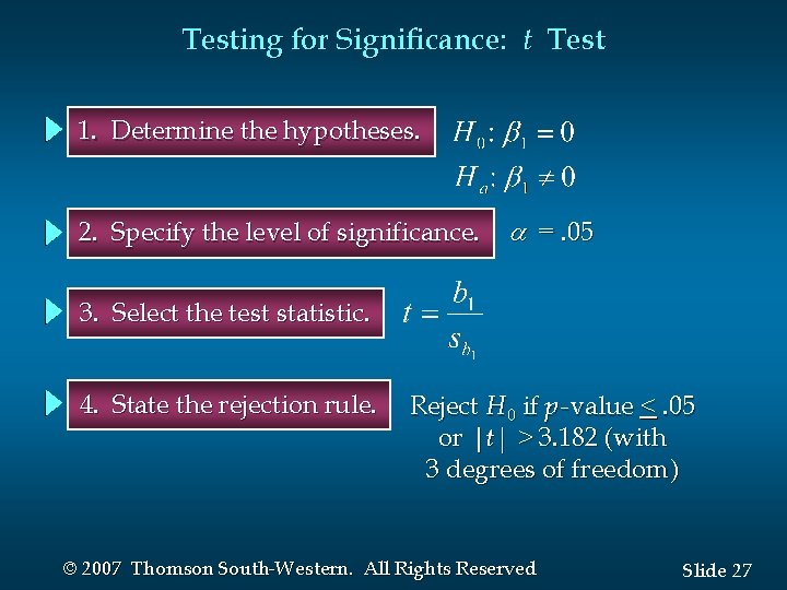
Testing for Significance: t Test 1. Determine the hypotheses. 2. Specify the level of significance. =. 05 3. Select the test statistic. 4. State the rejection rule. Reject H 0 if p -value <. 05 or |t| > 3. 182 (with 3 degrees of freedom) © 2007 Thomson South-Western. All Rights Reserved Slide 27

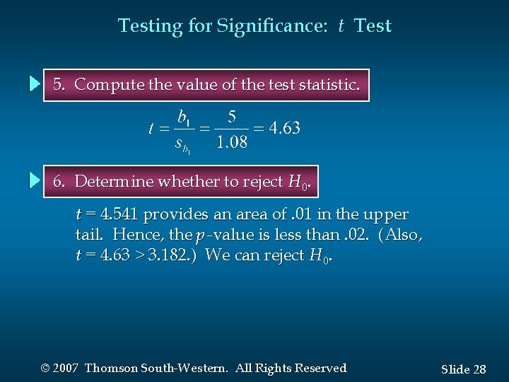
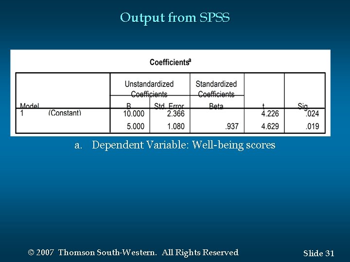
Testing for Significance: t Test 5. Compute the value of the test statistic. 6. Determine whether to reject H 0. t = 4. 541 provides an area of. 01 in the upper tail. Hence, the p -value is less than. 02. (Also, t = 4. 63 > 3. 182. ) We can reject H 0. © 2007 Thomson South-Western. All Rights Reserved Slide 28

Output for Example From SPSS a. Predictors: (Constant), Number of Counselling sessions © 2007 Thomson South-Western. All Rights Reserved Slide 29

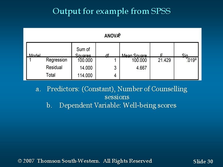
Output for example from SPSS a. Predictors: (Constant), Number of Counselling sessions b. Dependent Variable: Well-being scores © 2007 Thomson South-Western. All Rights Reserved Slide 30

Output from SPSS a. Dependent Variable: Well-being scores © 2007 Thomson South-Western. All Rights Reserved Slide 31

Confidence Interval for 1 n We can use a 95% confidence interval for 1 to test the hypotheses just used in the t test. n H 0 is rejected if the hypothesized value of 1 is not included in the confidence interval for 1. © 2007 Thomson South-Western. All Rights Reserved Slide 32

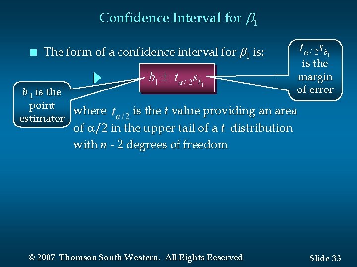
Confidence Interval for 1 n The form of a confidence interval for 1 is: b 1 is the point where estimator is the margin of error is the t value providing an area of a/2 in the upper tail of a t distribution with n - 2 degrees of freedom © 2007 Thomson South-Western. All Rights Reserved Slide 33

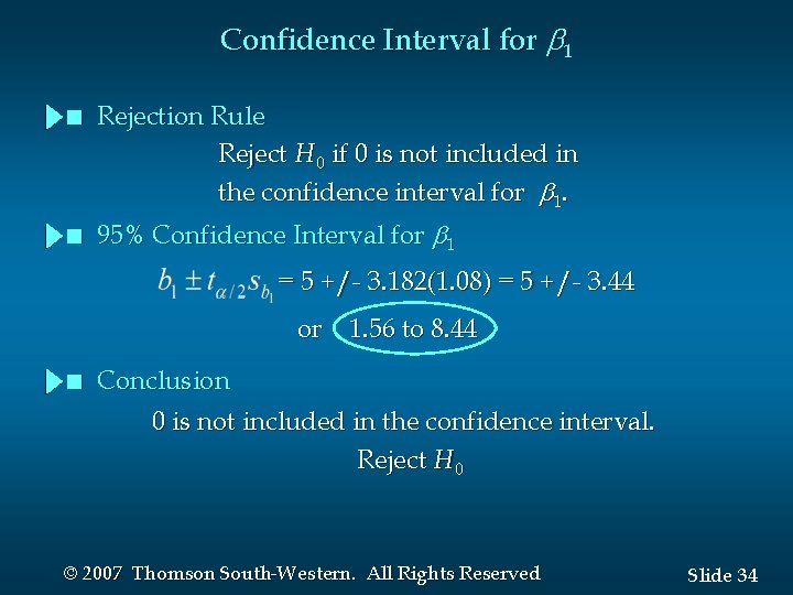
Confidence Interval for 1 n n Rejection Rule Reject H 0 if 0 is not included in the confidence interval for 1. 95% Confidence Interval for 1 = 5 +/- 3. 182(1. 08) = 5 +/- 3. 44 or 1. 56 to 8. 44 n Conclusion 0 is not included in the confidence interval. Reject H 0 © 2007 Thomson South-Western. All Rights Reserved Slide 34

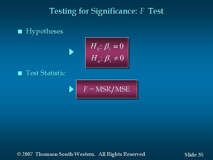
Testing for Significance: F Test n Hypotheses n Test Statistic F = MSR/MSE © 2007 Thomson South-Western. All Rights Reserved Slide 35

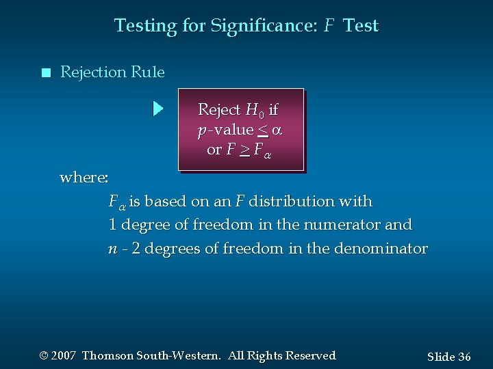
Testing for Significance: F Test n Rejection Rule Reject H 0 if p -value < a or F > F where: F is based on an F distribution with 1 degree of freedom in the numerator and n - 2 degrees of freedom in the denominator © 2007 Thomson South-Western. All Rights Reserved Slide 36

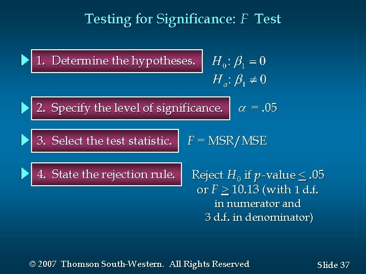
Testing for Significance: F Test 1. Determine the hypotheses. 2. Specify the level of significance. 3. Select the test statistic. 4. State the rejection rule. =. 05 F = MSR/MSE Reject H 0 if p -value <. 05 or F > 10. 13 (with 1 d. f. in numerator and 3 d. f. in denominator) © 2007 Thomson South-Western. All Rights Reserved Slide 37

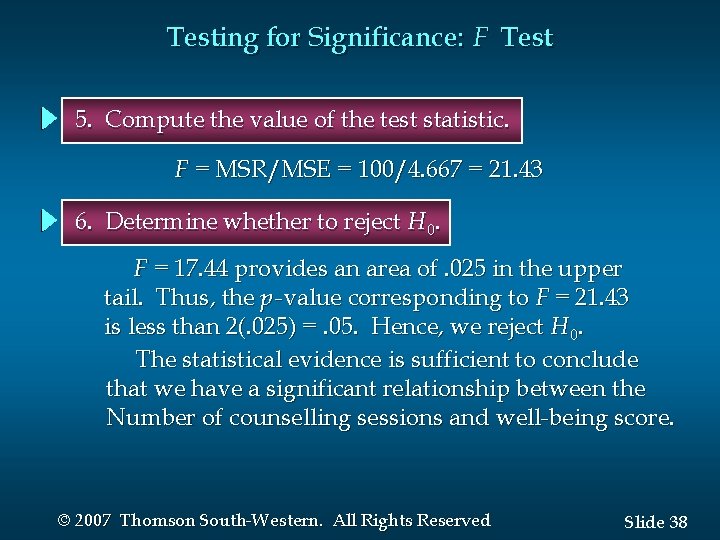
Testing for Significance: F Test 5. Compute the value of the test statistic. F = MSR/MSE = 100/4. 667 = 21. 43 6. Determine whether to reject H 0. F = 17. 44 provides an area of. 025 in the upper tail. Thus, the p -value corresponding to F = 21. 43 is less than 2(. 025) =. 05. Hence, we reject H 0. The statistical evidence is sufficient to conclude that we have a significant relationship between the Number of counselling sessions and well-being score. © 2007 Thomson South-Western. All Rights Reserved Slide 38

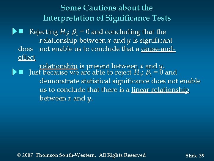
Some Cautions about the Interpretation of Significance Tests n Rejecting H 0: 1 = 0 and concluding that the relationship between x and y is significant does not enable us to conclude that a cause-andeffect relationship is present between x and y. n Just because we are able to reject H 0: 1 = 0 and demonstrate statistical significance does not enable us to conclude that there is a linear relationship between x and y. © 2007 Thomson South-Western. All Rights Reserved Slide 39