SIMILARITY SEARCH The Metric Space Approach Pavel Zezula

SIMILARITY SEARCH The Metric Space Approach Pavel Zezula, Giuseppe Amato, Vlastislav Dohnal, Michal Batko Similarity Search: Part I, Chapter 2

Table of Content Part I: Metric searching in a nutshell n Foundations of metric space searching n Survey of existing approaches Part II: Metric searching in large collections n Centralized index structures n Approximate similarity search n Parallel and distributed indexes Similarity Search: Part I, Chapter 2 2

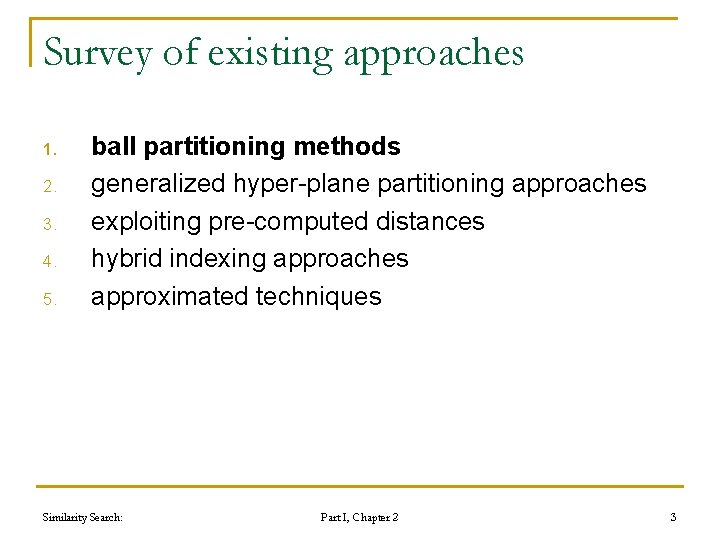
Survey of existing approaches 1. 2. 3. 4. 5. ball partitioning methods generalized hyper-plane partitioning approaches exploiting pre-computed distances hybrid indexing approaches approximated techniques Similarity Search: Part I, Chapter 2 3

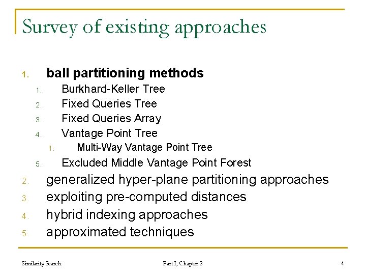
Survey of existing approaches ball partitioning methods 1. Burkhard-Keller Tree Fixed Queries Array Vantage Point Tree 1. 2. 3. 4. Multi-Way Vantage Point Tree 1. 5. 2. 3. 4. 5. Excluded Middle Vantage Point Forest generalized hyper-plane partitioning approaches exploiting pre-computed distances hybrid indexing approaches approximated techniques Similarity Search: Part I, Chapter 2 4

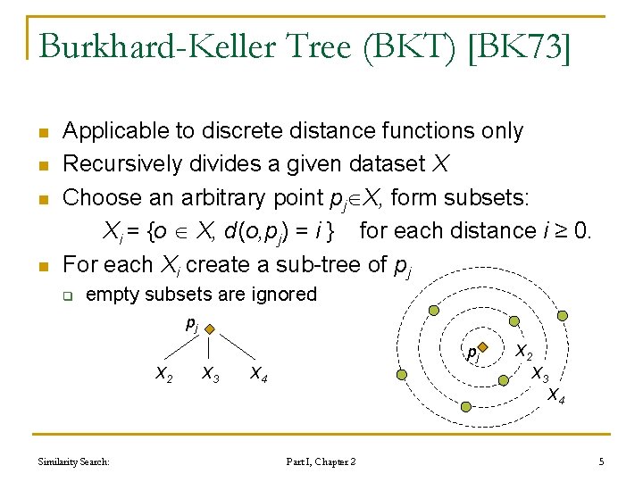
Burkhard-Keller Tree (BKT) [BK 73] n n Applicable to discrete distance functions only Recursively divides a given dataset X Choose an arbitrary point pj X, form subsets: Xi = {o X, d(o, pj) = i } for each distance i ≥ 0. For each Xi create a sub-tree of pj q empty subsets are ignored pj pj X 2 Similarity Search: X 3 X 4 Part I, Chapter 2 X 3 X 4 5

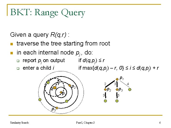
BKT: Range Query Given a query R(q, r) : n traverse the tree starting from root n in each internal node pj , do: q q report pj on output enter a child i if d(q, pj) ≤ r if max{d(q, pj) – r, 0} ≤ i ≤ d(q, pj) + r p 1 r q 2 p 2 3 p 2 p 1 3 4 p 3 5 p 3 Similarity Search: Part I, Chapter 2 6

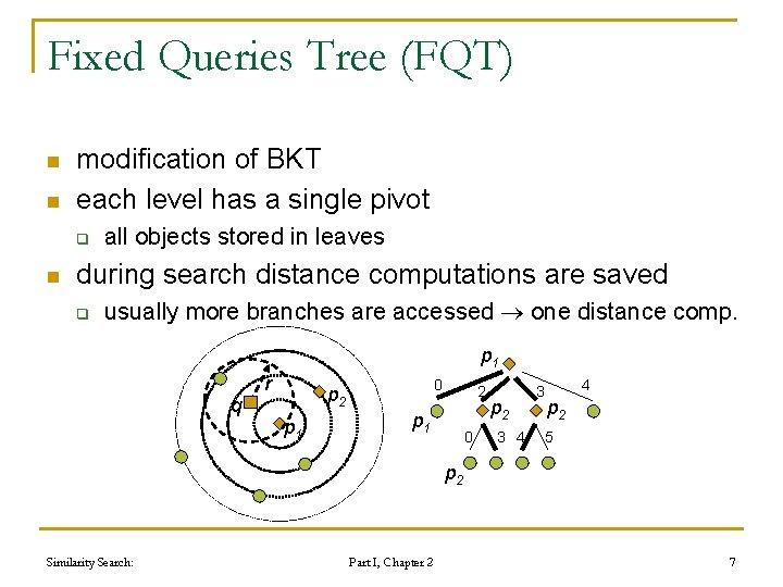
Fixed Queries Tree (FQT) n n modification of BKT each level has a single pivot q n all objects stored in leaves during search distance computations are saved q usually more branches are accessed one distance comp. p 1 r q 0 p 2 p 1 0 p 2 3 4 p 2 5 p 2 Similarity Search: Part I, Chapter 2 7

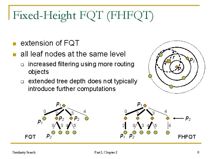
Fixed-Height FQT (FHFQT) n n extension of FQT all leaf nodes at the same level q q q increased filtering using more routing objects extended tree depth does not typically introduce further computations p 1 0 2 p 1 FQT Similarity Search: 0 p 2 3 4 r p 2 p 1 3 4 0 2 p 2 5 2 p 2 0 p 1 p 2 Part I, Chapter 2 3 3 4 5 4 p 2 6 FHFQT 8

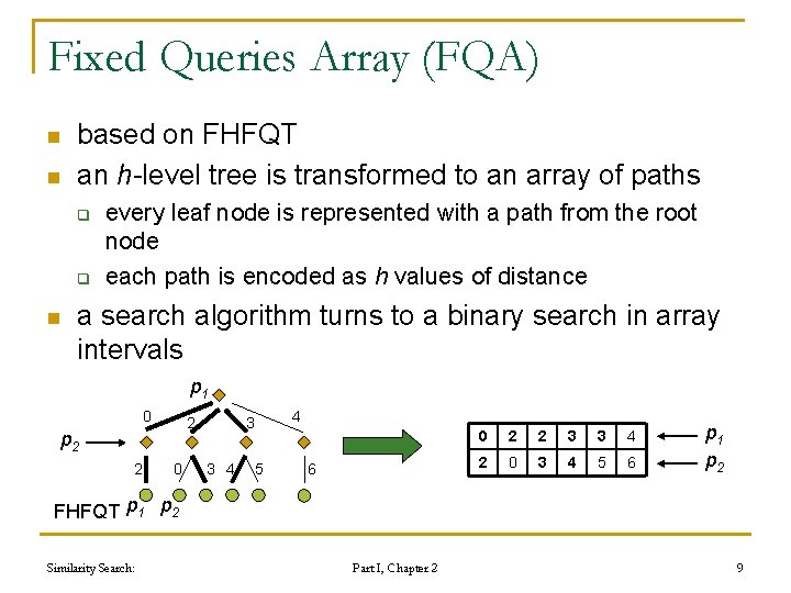
Fixed Queries Array (FQA) n n based on FHFQT an h-level tree is transformed to an array of paths q q n every leaf node is represented with a path from the root node each path is encoded as h values of distance a search algorithm turns to a binary search in array intervals p 1 0 2 p 2 2 0 3 3 4 5 4 6 0 2 2 3 3 4 2 0 3 4 5 6 p 1 p 2 FHFQT p 1 p 2 Similarity Search: Part I, Chapter 2 9

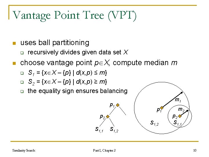
Vantage Point Tree (VPT) n uses ball partitioning q n recursively divides given data set X choose vantage point p X, compute median m q q q S 1 = {x X – {p} | d(x, p) ≤ m} S 2 = {x X – {p} | d(x, p) ≥ m} the equality sign ensures balancing p 1 p 2 S 1, 1 Similarity Search: S 1, 2 Part I, Chapter 2 m 1 p 1 S 1, 2 m 2 p 2 S 1, 1 10

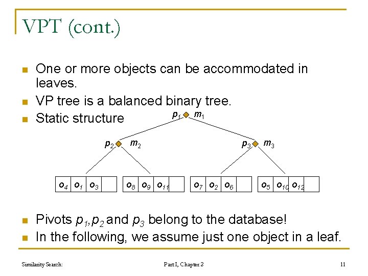
VPT (cont. ) n n n One or more objects can be accommodated in leaves. VP tree is a balanced binary tree. p 1 m 1 Static structure p 2 o 4 o 1 o 3 n n m 2 p 3 o 8 o 9 o 11 o 7 o 2 o 6 m 3 o 5 o 10 o 12 Pivots p 1, p 2 and p 3 belong to the database! In the following, we assume just one object in a leaf. Similarity Search: Part I, Chapter 2 11

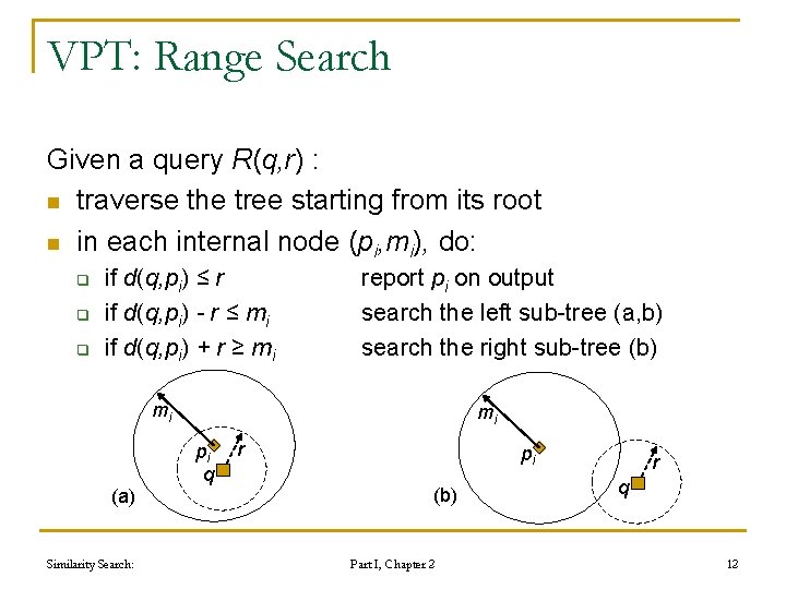
VPT: Range Search Given a query R(q, r) : n traverse the tree starting from its root n in each internal node (pi, mi), do: q q q if d(q, pi) ≤ r if d(q, pi) - r ≤ mi if d(q, pi) + r ≥ mi report pi on output search the left sub-tree (a, b) search the right sub-tree (b) mi (a) Similarity Search: mi pi q r pi (b) Part I, Chapter 2 r q 12

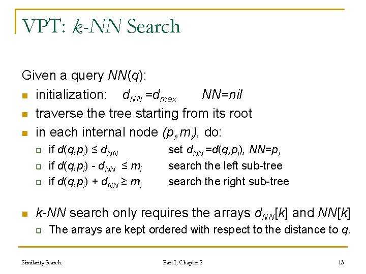
VPT: k-NN Search Given a query NN(q): n initialization: d. NN =dmax NN=nil n traverse the tree starting from its root n in each internal node (pi, mi), do: q q q n if d(q, pi) ≤ d. NN if d(q, pi) - d. NN ≤ mi if d(q, pi) + d. NN ≥ mi set d. NN =d(q, pi), NN=pi search the left sub-tree search the right sub-tree k-NN search only requires the arrays d. NN[k] and NN[k] q The arrays are kept ordered with respect to the distance to q. Similarity Search: Part I, Chapter 2 13

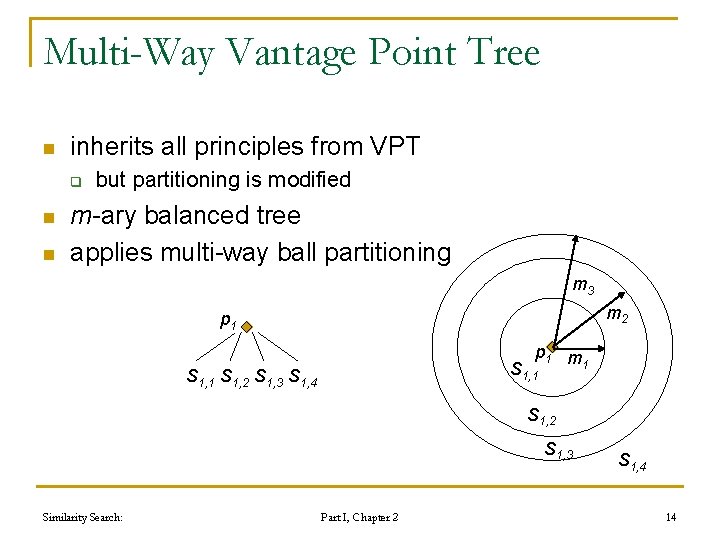
Multi-Way Vantage Point Tree n inherits all principles from VPT q n n but partitioning is modified m-ary balanced tree applies multi-way ball partitioning m 3 m 2 p 1 m 1 S 1, 2 S 1, 3 S 1, 4 S 1, 2 S 1, 3 Similarity Search: Part I, Chapter 2 S 1, 4 14

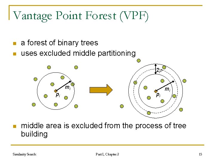
Vantage Point Forest (VPF) n n a forest of binary trees uses excluded middle partitioning 2 mi pi n pi mi middle area is excluded from the process of tree building Similarity Search: Part I, Chapter 2 15

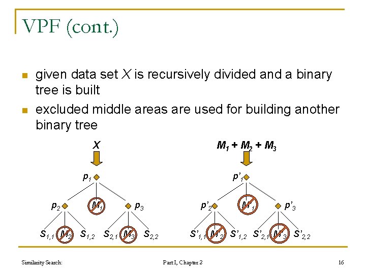
VPF (cont. ) n n given data set X is recursively divided and a binary tree is built excluded middle areas are used for building another binary tree X M 1 + M 2 + M 3 p 1 p 2 S 1, 1 M 2 Similarity Search: p’ 1 M 1 S 1, 2 S 2, 1 M 3 p’ 2 S 2, 2 M’ 1 p’ 3 S’ 1, 1 M’ 2 S’ 1, 2 S’ 2, 1 M’ 3 S’ 2, 2 Part I, Chapter 2 16

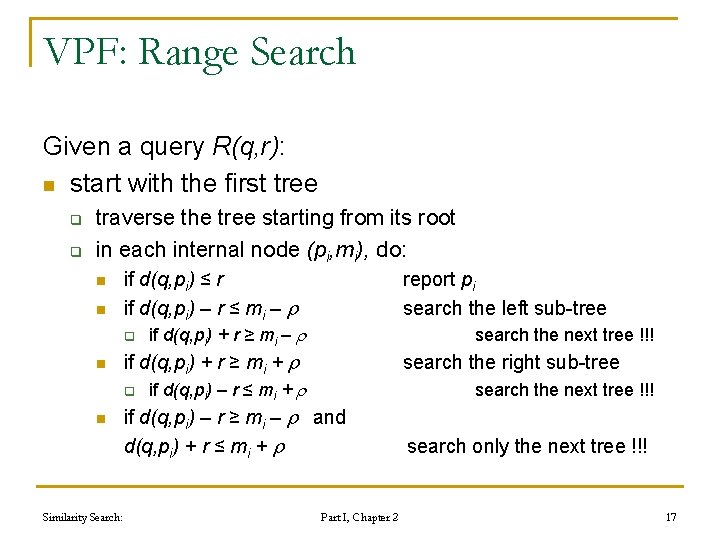
VPF: Range Search Given a query R(q, r): n start with the first tree q q traverse the tree starting from its root in each internal node (pi, mi), do: n n Similarity Search: if d(q, pi) ≤ r if d(q, pi) – r ≤ mi – q if d(q, pi) + r ≥ mi – if d(q, pi) + r ≥ mi + q if d(q, pi) – r ≤ mi + if d(q, pi) – r ≥ mi – and d(q, pi) + r ≤ mi + Part I, Chapter 2 report pi search the left sub-tree search the next tree !!! search the right sub-tree search the next tree !!! search only the next tree !!! 17

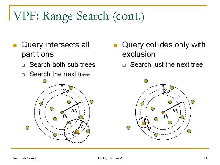
VPF: Range Search (cont. ) n Query intersects all partitions q q n Search both sub-trees Search the next tree Query collides only with exclusion q Search just the next tree 2 pi 2 mi pi r q q Similarity Search: mi Part I, Chapter 2 18

Survey of existing approaches ball partitioning methods generalized hyper-plane partitioning approaches 1. 2. 3. 4. 5. Bisector Tree Generalized Hyper-plane Tree exploiting pre-computed distances hybrid indexing approaches approximated techniques Similarity Search: Part I, Chapter 2 19

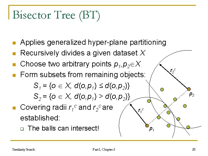
Bisector Tree (BT) n n n Applies generalized hyper-plane partitioning Recursively divides a given dataset X Choose two arbitrary points p 1, p 2 X Form subsets from remaining objects: S 1 = {o X, d(o, p 1) ≤ d(o, p 2)} S 2 = {o X, d(o, p 1) > d(o, p 2)} Covering radii r 1 c and r 2 c are r 1 c established: q The balls can intersect! Similarity Search: Part I, Chapter 2 c p 2 p 1 20

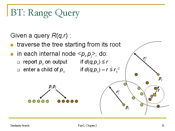
BT: Range Query Given a query R(q, r) : n traverse the tree starting from its root n in each internal node <pi, pj>, do: q q report px on output enter a child of px rjc if d(q, px) ≤ r if d(q, px) – r ≤ rxc pj pi pj r ric q pi Similarity Search: Part I, Chapter 2 21

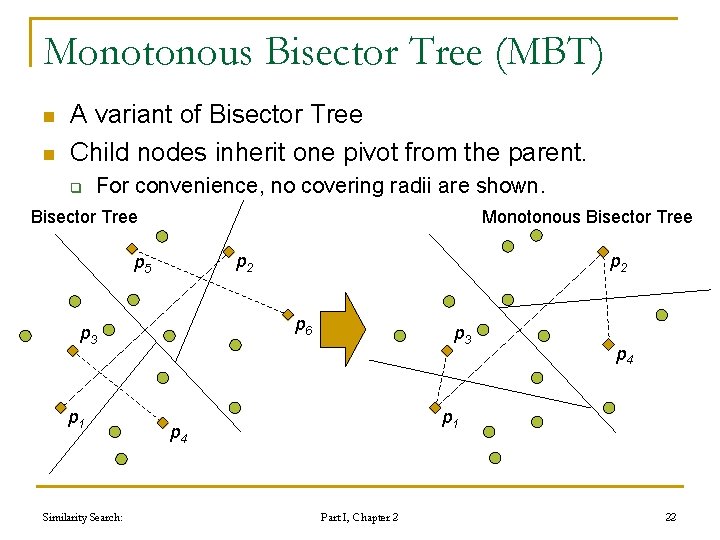
Monotonous Bisector Tree (MBT) n n A variant of Bisector Tree Child nodes inherit one pivot from the parent. q For convenience, no covering radii are shown. Bisector Tree Monotonous Bisector Tree p 2 p 5 p 6 p 3 p 1 Similarity Search: p 2 p 3 p 4 p 1 p 4 Part I, Chapter 2 22

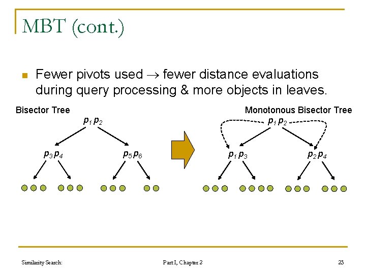
MBT (cont. ) n Fewer pivots used fewer distance evaluations during query processing & more objects in leaves. Bisector Tree p 3 p 4 Similarity Search: Monotonous Bisector Tree p 1 p 2 p 5 p 6 p 1 p 3 Part I, Chapter 2 p 4 23

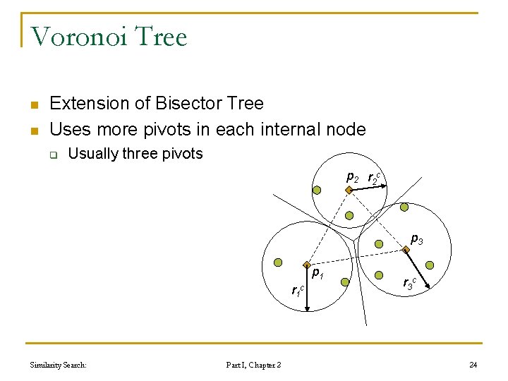
Voronoi Tree n n Extension of Bisector Tree Uses more pivots in each internal node q Usually three pivots p 2 r 2 c p 3 p 1 r 1 Similarity Search: Part I, Chapter 2 c r 3 c 24

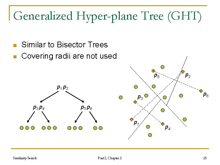
Generalized Hyper-plane Tree (GHT) n n Similar to Bisector Trees Covering radii are not used p 2 p 5 p 1 p 2 p 6 p 3 p 4 p 5 p 6 p 1 Similarity Search: Part I, Chapter 2 p 4 25

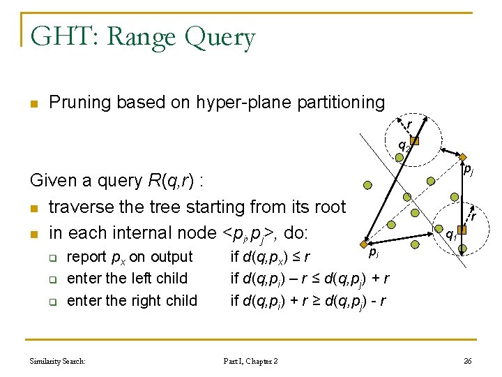
GHT: Range Query n Pruning based on hyper-plane partitioning r q 2 Given a query R(q, r) : n traverse the tree starting from its root n in each internal node <pi, pj>, do: q q q report px on output enter the left child enter the right child Similarity Search: pj r q 1 pi if d(q, px) ≤ r if d(q, pi) – r ≤ d(q, pj) + r if d(q, pi) + r ≥ d(q, pj) - r Part I, Chapter 2 26

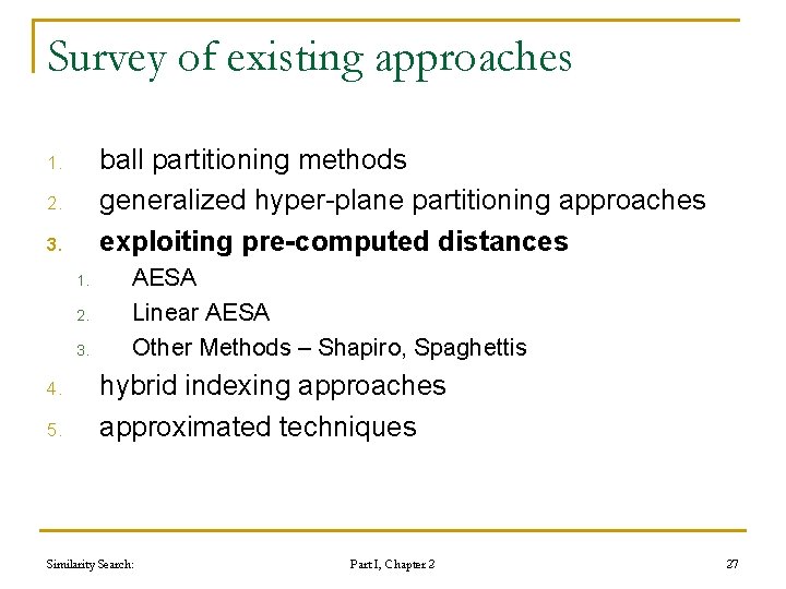
Survey of existing approaches ball partitioning methods generalized hyper-plane partitioning approaches exploiting pre-computed distances 1. 2. 3. 4. 5. AESA Linear AESA Other Methods – Shapiro, Spaghettis hybrid indexing approaches approximated techniques Similarity Search: Part I, Chapter 2 27

Exploiting Pre-computed Distances n During insertion of an object into a structure some distances are evaluated n If they are remembered, we can employ them in filtering when processing a query Similarity Search: Part I, Chapter 2 28

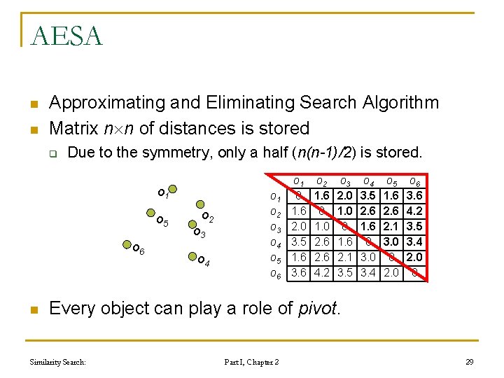
AESA n n Approximating and Eliminating Search Algorithm Matrix n n of distances is stored q Due to the symmetry, only a half (n(n-1)/2) is stored. o 1 o 5 o 6 n o 2 o 3 o 4 o 1 o 2 o 3 o 4 o 5 o 6 o 1 0 1. 6 2. 0 3. 5 1. 6 3. 6 o 2 1. 6 0 1. 0 2. 6 4. 2 o 3 2. 0 1. 0 0 1. 6 2. 1 3. 5 o 4 3. 5 2. 6 1. 6 0 3. 4 o 5 1. 6 2. 1 3. 0 0 2. 0 o 6 3. 6 4. 2 3. 5 3. 4 2. 0 0 Every object can play a role of pivot. Similarity Search: Part I, Chapter 2 29

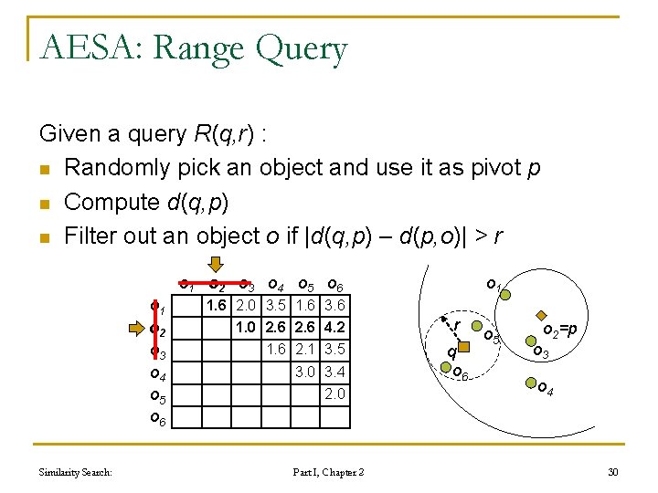
AESA: Range Query Given a query R(q, r) : n Randomly pick an object and use it as pivot p n Compute d(q, p) n Filter out an object o if |d(q, p) – d(p, o)| > r o 1 o 2 o 3 o 4 o 5 o 6 Similarity Search: 1. 6 2. 0 3. 5 1. 6 3. 6 1. 0 2. 6 4. 2 1. 6 2. 1 3. 5 3. 0 3. 4 2. 0 Part I, Chapter 2 r q o 6 o 5 o 2=p o 3 o 4 30

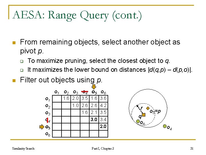
AESA: Range Query (cont. ) n From remaining objects, select another object as pivot p. q q n To maximize pruning, select the closest object to q. It maximizes the lower bound on distances |d(q, p) – d(p, o)|. Filter out objects using p. o 1 o 2 o 3 o 4 o 5 o 6 Similarity Search: 1. 6 2. 0 3. 5 1. 6 3. 6 1. 0 2. 6 4. 2 1. 6 2. 1 3. 5 3. 0 3. 4 2. 0 Part I, Chapter 2 r q o 6 o 5=p o 4 31

AESA: Range Query (cont. ) n This process is repeated until the number of remaining objects is small enough q n o 1 o 2 o 3 o 4 o 5 o 6 Check remaining objects directly with q. q n Or all objects have been used as pivots. Report o if d(q, o) ≤ r. r q o 6 o 5 o 1 o 2 o 3 o 4 o 5 o 6 1. 6 2. 0 3. 5 1. 6 3. 6 1. 0 2. 6 4. 2 1. 6 2. 1 3. 5 3. 0 3. 4 2. 0 Objects o that fulfill d(q, p)+d(p, o) ≤ r can directly be reported on the output without further checking. q E. g. o 5, because it was the pivot in the previous step. Similarity Search: Part I, Chapter 2 32

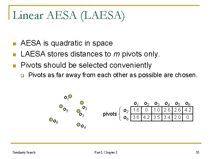
Linear AESA (LAESA) n n n AESA is quadratic in space LAESA stores distances to m pivots only. Pivots should be selected conveniently q Pivots as far away from each other as possible are chosen. o 1 o 5 o 6 Similarity Search: o 2 o 3 o 1 pivots o 2 o 3 o 4 o 5 o 6 o 2 1. 6 0 1. 0 2. 6 4. 2 o 6 3. 6 4. 2 3. 5 3. 4 2. 0 0 o 4 Part I, Chapter 2 33

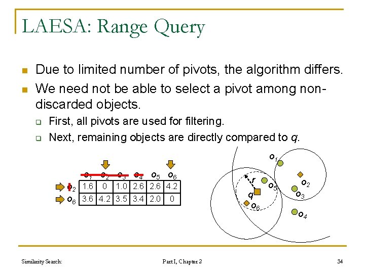
LAESA: Range Query n n Due to limited number of pivots, the algorithm differs. We need not be able to select a pivot among nondiscarded objects. q q First, all pivots are used for filtering. Next, remaining objects are directly compared to q. o 1 o 2 o 3 o 4 o 5 o 6 o 2 1. 6 0 1. 0 2. 6 4. 2 o 6 3. 6 4. 2 3. 5 3. 4 2. 0 0 Similarity Search: Part I, Chapter 2 r q o 6 o 5 o 2 o 3 o 4 34

LAESA: Summary n AESA and LAESA tend to be linear in distance computations q For larger query radii or higher values of k Similarity Search: Part I, Chapter 2 35

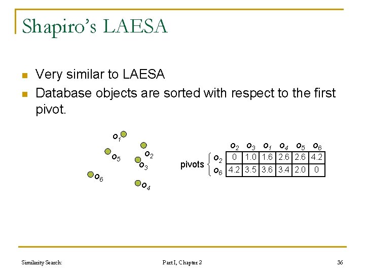
Shapiro’s LAESA n n Very similar to LAESA Database objects are sorted with respect to the first pivot. o 1 o 5 o 6 Similarity Search: o 2 o 3 o 1 o 4 o 5 o 6 pivots o 2 0 1. 6 2. 6 4. 2 o 6 4. 2 3. 5 3. 6 3. 4 2. 0 0 o 4 Part I, Chapter 2 36

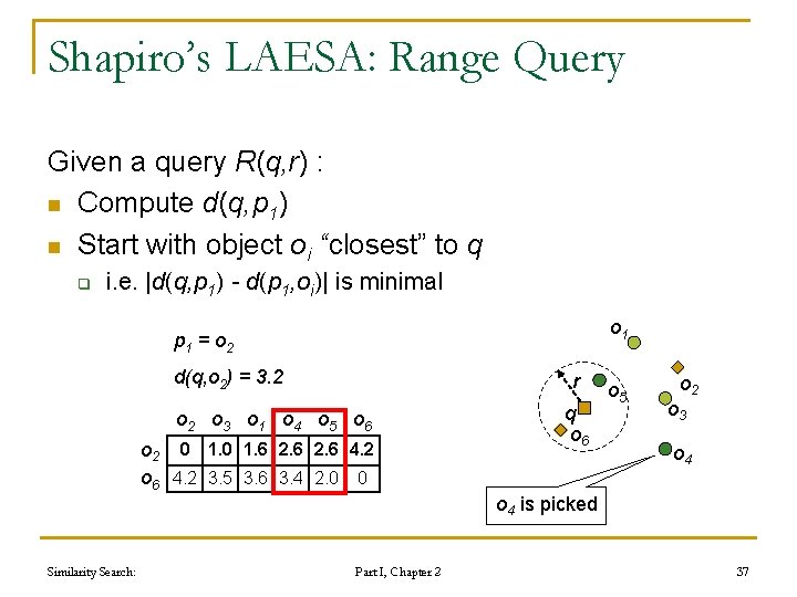
Shapiro’s LAESA: Range Query Given a query R(q, r) : n Compute d(q, p 1) n Start with object oi “closest” to q q i. e. |d(q, p 1) - d(p 1, oi)| is minimal o 1 p 1 = o 2 d(q, o 2) = 3. 2 r o 2 o 3 o 1 o 4 o 5 o 6 o 2 0 1. 6 2. 6 4. 2 o 6 4. 2 3. 5 3. 6 3. 4 2. 0 0 q o 6 o 5 o 2 o 3 o 4 is picked Similarity Search: Part I, Chapter 2 37

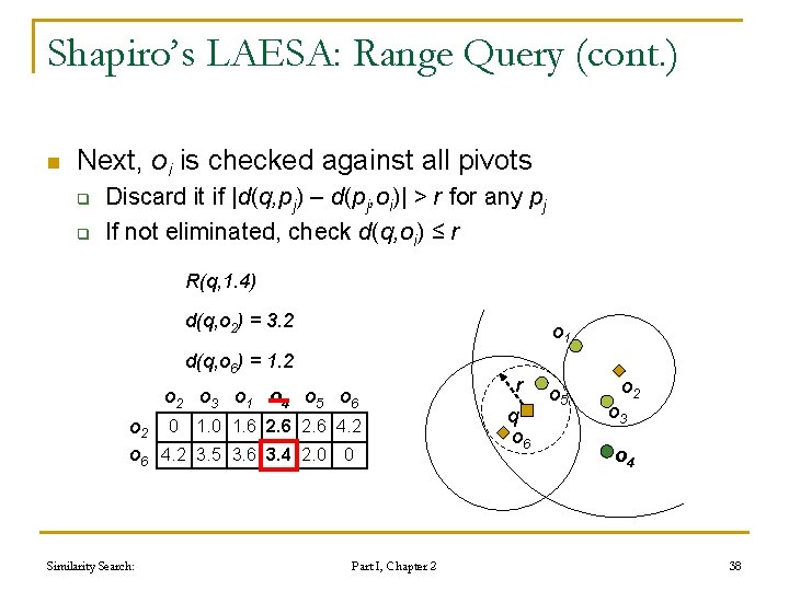
Shapiro’s LAESA: Range Query (cont. ) n Next, oi is checked against all pivots q q Discard it if |d(q, pj) – d(pj, oi)| > r for any pj If not eliminated, check d(q, oi) ≤ r R(q, 1. 4) d(q, o 2) = 3. 2 o 1 d(q, o 6) = 1. 2 o 3 o 1 o 4 o 5 o 6 o 2 0 1. 6 2. 6 4. 2 o 6 4. 2 3. 5 3. 6 3. 4 2. 0 0 Similarity Search: Part I, Chapter 2 r q o 6 o 5 o 2 o 3 o 4 38

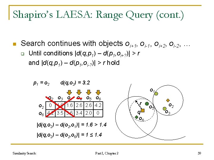
Shapiro’s LAESA: Range Query (cont. ) n Search continues with objects oi+1, oi-1, oi+2, oi-2, … q Until conditions |d(q, p 1) – d(p 1, oi+? )| > r and |d(q, p 1) – d(p 1, oi-? )| > r hold p 1 = o 2 d(q, o 2) = 3. 2 o 1 o 2 o 3 o 1 o 4 o 5 o 6 o 2 0 1. 6 2. 6 4. 2 o 6 4. 2 3. 5 3. 6 3. 4 2. 0 0 |d(q, o 2) – d(o 2, o 1)| = 1. 6 > 1. 4 r q o 6 o 5 o 2 o 3 |d(q, o 2) – d(o 2, o 6)| = 1 ≤ 1. 4 Similarity Search: Part I, Chapter 2 39

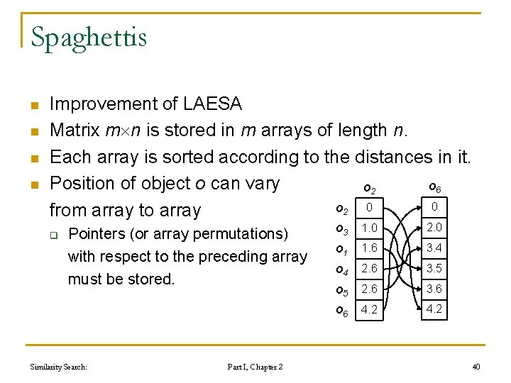
Spaghettis n n Improvement of LAESA Matrix m n is stored in m arrays of length n. Each array is sorted according to the distances in it. Position of object o can vary o 6 o 2 0 from array to array q Pointers (or array permutations) with respect to the preceding array must be stored. Similarity Search: Part I, Chapter 2 o 3 1. 0 2. 0 o 1 1. 6 3. 4 o 4 2. 6 3. 5 o 5 2. 6 3. 6 o 6 4. 2 40

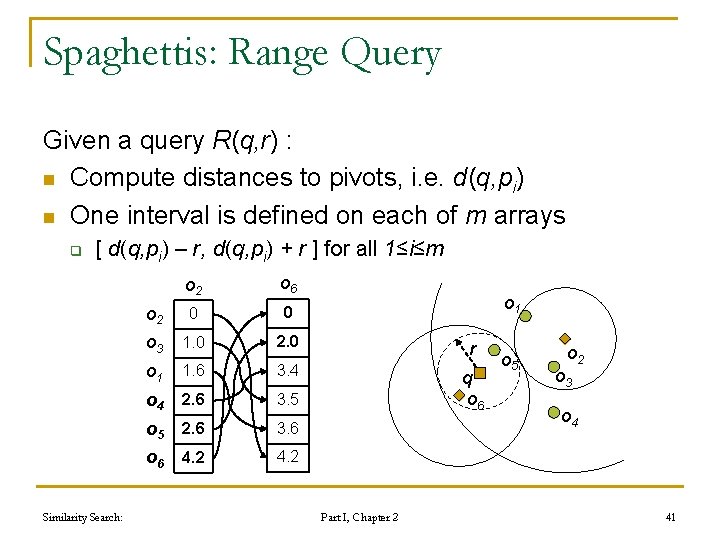
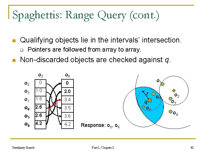
Spaghettis: Range Query Given a query R(q, r) : n Compute distances to pivots, i. e. d(q, pi) n One interval is defined on each of m arrays q [ d(q, pi) – r, d(q, pi) + r ] for all 1≤i≤m Similarity Search: o 2 o 6 o 2 0 0 o 3 1. 0 2. 0 r o 1 1. 6 3. 4 o 4 2. 6 3. 5 q o 6 o 5 2. 6 3. 6 o 6 4. 2 o 1 Part I, Chapter 2 o 5 o 2 o 3 o 4 41

Spaghettis: Range Query (cont. ) n Qualifying objects lie in the intervals’ intersection. q n Pointers are followed from array to array. Non-discarded objects are checked against q. o 2 o 6 o 2 0 0 o 3 1. 0 o 1 2. 0 1. 6 r 3. 4 o 4 2. 6 3. 5 q o 6 o 5 2. 6 3. 6 o 6 4. 2 Similarity Search: o 5 o 2 o 3 o 4 Response: o 5, o 6 Part I, Chapter 2 42

Survey of existing approaches ball partitioning methods generalized hyper-plane partitioning approaches exploiting pre-computed distances hybrid indexing approaches 1. 2. 3. 4. 5. Multi Vantage Point Tree Geometric Near-neighbor Access Tree Spatial Approximation Tree M-tree Similarity Hashing approximated techniques Similarity Search: Part I, Chapter 2 43

Introduction n Structures that store pre-computed distances have high space requirements q n But good performance boost during query processing. Hybrid approaches combine partitioning and precomputed distances into a single system q q Less space requirements Good query performance Similarity Search: Part I, Chapter 2 44

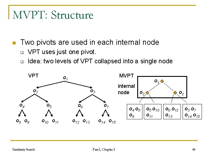
Multi Vantage Point Tree (MVPT) n Based on Vantage Point Tree (VPT) q n Tries to decrease the number of pivots q n These distances are evaluated during insertion of objects. No object duplication q n With the aim of improving performance in terms of distance computations. Stores distances to pivots in leaves q n Targeted to static collections as well. Objects playing the role of a pivot are stored only in internal nodes. Leaf nodes can contain more than one object. Similarity Search: Part I, Chapter 2 45

MVPT: Structure n Two pivots are used in each internal node q q VPT uses just one pivot. Idea: two levels of VPT collapsed into a single node VPT MVPT o 1 o 2 internal o 2 node o 3 o 4 o 5 o 6 o 7 o 8 o 9 o 10 o 11 o 12 o 13 o 14 o 15 Similarity Search: Part I, Chapter 2 o 4 o 8 o 9 o 1 o 2 o 5 o 10 o 11 o 6 o 12 o 13 o 7 o 14 o 15 46

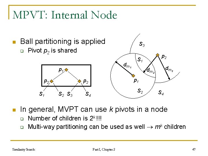
MPVT: Internal Node n Ball partitioning is applied q Pivot p 2 is shared dm 1 p 2 S 1 n S 3 dm 2 p 1 p 2 S 3 p 2 S 1 S 2 S 4 In general, MVPT can use k pivots in a node q q Number of children is 2 k !!! Multi-way partitioning can be used as well mk children Similarity Search: Part I, Chapter 2 47

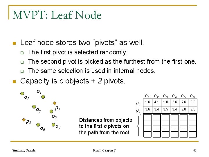
MVPT: Leaf Node n Leaf node stores two “pivots” as well. q q q n The first pivot is selected randomly, The second pivot is picked as the furthest from the first one. The same selection is used in internal nodes. Capacity is c objects + 2 pivots. o 2 o 1 o 5 p 2 o 6 Similarity Search: p 1 o 3 o 4 Distances from objects to the first h pivots on the path from the root Part I, Chapter 2 o 1 o 2 o 3 o 4 o 5 o 6 p 1 1. 6 4. 1 1. 0 2. 6 3. 3 p 2 3. 6 3. 4 3. 5 3. 4 2. 0 2. 5 … … … 48

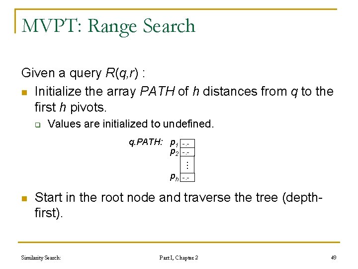
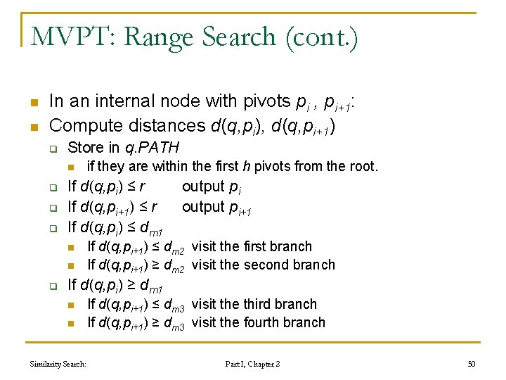
MVPT: Range Search Given a query R(q, r) : n Initialize the array PATH of h distances from q to the first h pivots. q Values are initialized to undefined. -. -. - ph -. - … q. PATH: p 1 p 2 n Start in the root node and traverse the tree (depthfirst). Similarity Search: Part I, Chapter 2 49

MVPT: Range Search (cont. ) n n In an internal node with pivots pi , pi+1: Compute distances d(q, pi), d(q, pi+1) q Store in q. PATH n q q q If d(q, pi) ≤ r If d(q, pi+1) ≤ r If d(q, pi) ≤ dm 1 n n q if they are within the first h pivots from the root. output pi+1 If d(q, pi+1) ≤ dm 2 visit the first branch If d(q, pi+1) ≥ dm 2 visit the second branch If d(q, pi) ≥ dm 1 n n Similarity Search: If d(q, pi+1) ≤ dm 3 visit the third branch If d(q, pi+1) ≥ dm 3 visit the fourth branch Part I, Chapter 2 50

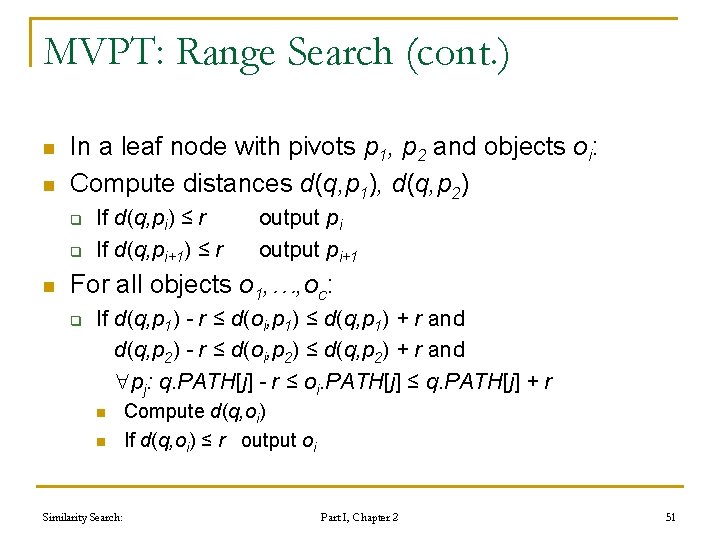
MVPT: Range Search (cont. ) n n In a leaf node with pivots p 1, p 2 and objects oi: Compute distances d(q, p 1), d(q, p 2) q q n If d(q, pi) ≤ r If d(q, pi+1) ≤ r output pi+1 For all objects o 1, …, oc: q If d(q, p 1) - r ≤ d(oi, p 1) ≤ d(q, p 1) + r and d(q, p 2) - r ≤ d(oi, p 2) ≤ d(q, p 2) + r and pj: q. PATH[j] - r ≤ oi. PATH[j] ≤ q. PATH[j] + r n n Similarity Search: Compute d(q, oi) If d(q, oi) ≤ r output oi Part I, Chapter 2 51

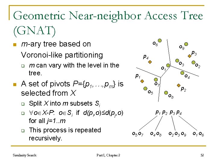
Geometric Near-neighbor Access Tree (GNAT) n m-ary tree based on Voronoi-like partitioning q n m can vary with the level in the tree. A set of pivots P={p 1, …, pm} is selected from X q q q Split X into m subsets Si o X-P: o Si if d(pi, o)≤d(pj, o) for all j=1. . m This process is repeated recursively. Similarity Search: Part I, Chapter 2 o 6 o 9 p 4 p 3 o 1 p 1 o 2 o 4 o 7 o 5 p 2 o 8 p 1 p 2 p 3 p 4 o 5 o 7 o 4 o 8 o 2 o 3 o 9 o 1 o 6 52

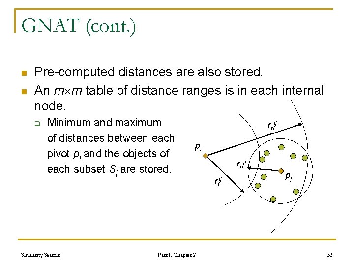
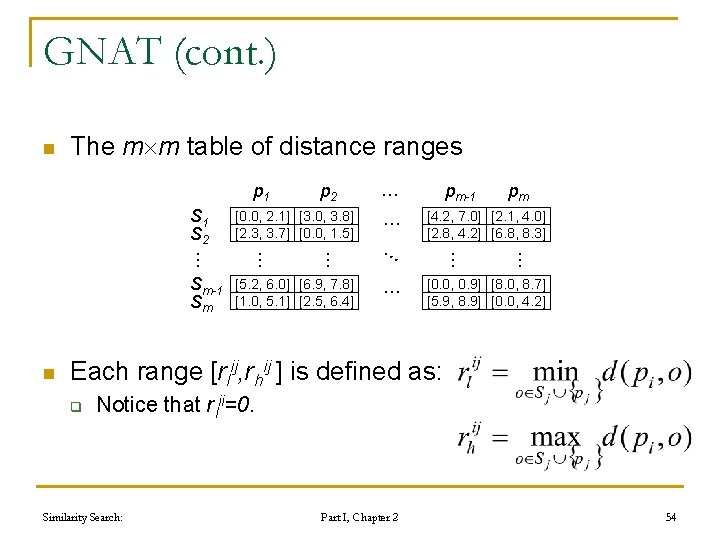
GNAT (cont. ) n n Pre-computed distances are also stored. An m m table of distance ranges is in each internal node. q Minimum and maximum of distances between each pivot pi and the objects of each subset Sj are stored. Similarity Search: rhij pi Part I, Chapter 2 rhjj rlij pj 53

GNAT (cont. ) n The m m table of distance ranges p 1 S 2 … … … pm-1 pm [4. 2, 7. 0] [2. 1, 4. 0] [2. 8, 4. 2] [6. 8, 8. 3] … [5. 2, 6. 0] [6. 9, 7. 8] [1. 0, 5. 1] [2. 5, 6. 4] … … … n [0. 0, 2. 1] [3. 0, 3. 8] [2. 3, 3. 7] [0. 0, 1. 5] … … Sm-1 Sm p 2 [0. 0, 0. 9] [8. 0, 8. 7] [5. 9, 8. 9] [0. 0, 4. 2] Each range [rlij, rhij ] is defined as: q Notice that rlii=0. Similarity Search: Part I, Chapter 2 54

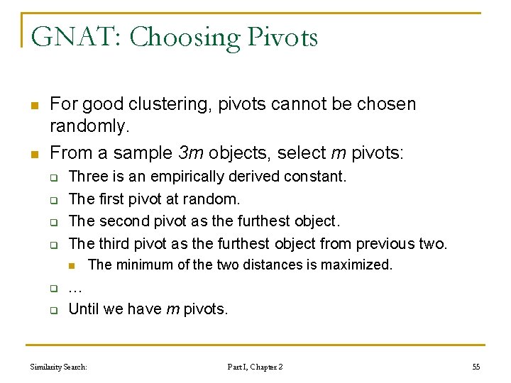
GNAT: Choosing Pivots n n For good clustering, pivots cannot be chosen randomly. From a sample 3 m objects, select m pivots: q q Three is an empirically derived constant. The first pivot at random. The second pivot as the furthest object. The third pivot as the furthest object from previous two. n q q The minimum of the two distances is maximized. … Until we have m pivots. Similarity Search: Part I, Chapter 2 55

GNAT: Range Search Given a query R(q, r) : n Start in the root node and traverse the tree (depthfirst). n In internal nodes, employ the distance ranges to prune some branches. n In leaf nodes, all objects are directly compared to q. q If d(q, o)≤ r , report o to the output. Similarity Search: Part I, Chapter 2 56

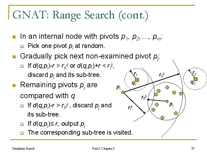
GNAT: Range Search (cont. ) n In an internal node with pivots p 1, p 2, …, pm: q n Gradually pick next non-examined pivot pj: q n Pick one pivot pi at random. If d(q, pi)-r > rhij or d(q, pi)+r < rlij, discard pj and its sub-tree. Remaining pivots pj are compared with q q r 1 pi Part I, Chapter 2 q 1 If d(q, pi)-r > rhjj , discard pj and rlij its sub-tree. If d(q, pj)≤ r, output pj The corresponding sub-tree is visited. Similarity Search: r 2 rhij rhjj pj 57

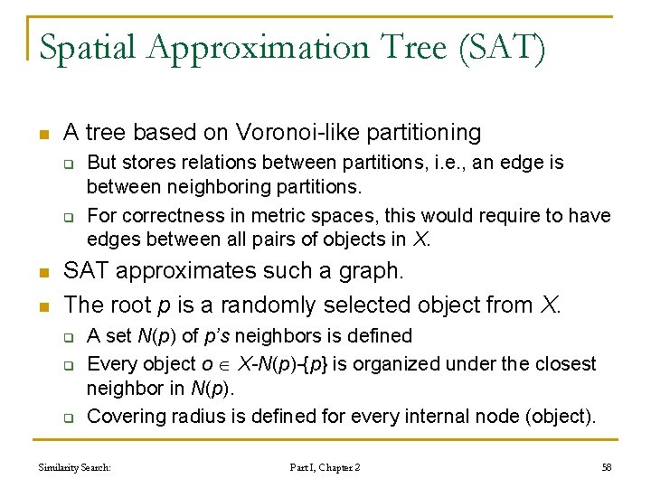
Spatial Approximation Tree (SAT) n A tree based on Voronoi-like partitioning q q n n But stores relations between partitions, i. e. , an edge is between neighboring partitions. For correctness in metric spaces, this would require to have edges between all pairs of objects in X. SAT approximates such a graph. The root p is a randomly selected object from X. q q q A set N(p) of p’s neighbors is defined Every object o X-N(p)-{p} is organized under the closest neighbor in N(p). Covering radius is defined for every internal node (object). Similarity Search: Part I, Chapter 2 58

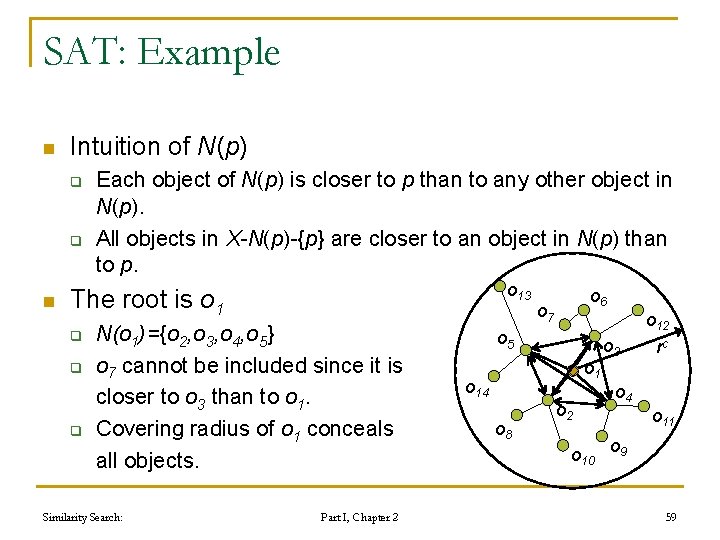
SAT: Example n Intuition of N(p) q q n Each object of N(p) is closer to p than to any other object in N(p). All objects in X-N(p)-{p} are closer to an object in N(p) than to p. o 13 The root is o 1 q q q N(o 1)={o 2, o 3, o 4, o 5} o 7 cannot be included since it is closer to o 3 than to o 1. Covering radius of o 1 conceals all objects. Similarity Search: Part I, Chapter 2 o 6 o 7 o 12 o 5 o 14 o 8 o 2 o 10 o 3 rc o 4 o 11 o 9 59

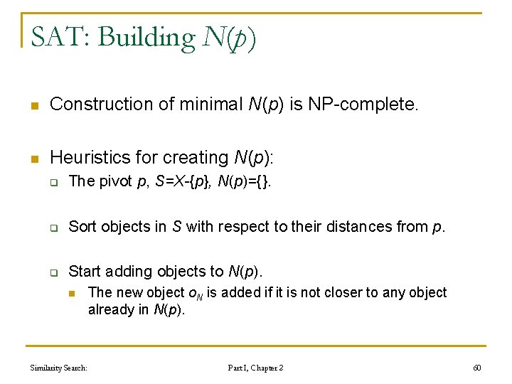
SAT: Building N(p ) n Construction of minimal N(p) is NP-complete. n Heuristics for creating N(p): q The pivot p, S=X-{p}, N(p)={}. q Sort objects in S with respect to their distances from p. q Start adding objects to N(p). n Similarity Search: The new object o. N is added if it is not closer to any object already in N(p). Part I, Chapter 2 60

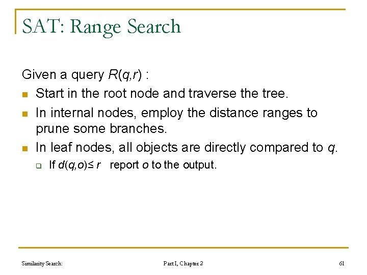
SAT: Range Search Given a query R(q, r) : n Start in the root node and traverse the tree. n In internal nodes, employ the distance ranges to prune some branches. n In leaf nodes, all objects are directly compared to q. q If d(q, o)≤ r report o to the output. Similarity Search: Part I, Chapter 2 61

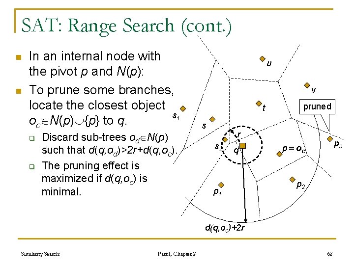
SAT: Range Search (cont. ) n n In an internal node with the pivot p and N(p): To prune some branches, locate the closest object s 1 oc N(p) {p} to q. q q Discard sub-trees od N(p) such that d(q, od)>2 r+d(q, oc). The pruning effect is maximized if d(q, oc) is minimal. u v t s pruned r s 2 q p 1 p 3 p = oc p 2 d(q, oc)+2 r Similarity Search: Part I, Chapter 2 62

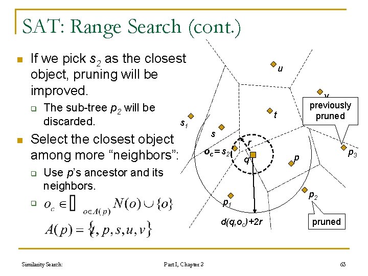
SAT: Range Search (cont. ) n If we pick s 2 as the closest object, pruning will be improved. q n The sub-tree p 2 will be discarded. s oc = s 2 r q Use p’s ancestor and its neighbors. p 1 q d(q, oc)+2 r Similarity Search: v previously pruned t s 1 Select the closest object among more “neighbors”: q u Part I, Chapter 2 p 3 p p 2 pruned 63

SAT: Range Search (cont. ) n Finally, apply covering radii of remaining objects q Discard od such that d(q, od)>rdc+r. Similarity Search: Part I, Chapter 2 64

M-tree n n n n inherently dynamic structure disk-oriented (fixed-size nodes) built in a bottom-up fashion each node constrained by a sphere-like (ball) region leaf node: data objects + their distances from a pivot kept in the parent node internal node: pivot + radius covering the subtree, distance from the pivot the parent pivot filtering: covering radii + pre-computed distances Similarity Search: Part I, Chapter 2 65

M-tree: Extensions n bulk-loading algorithm q q q n Slim-tree q q q n considers the trade-off: dynamic properties vs. performance M-tree building algorithm for a dataset given in advance results in more efficient M-tree variant of M-tree (dynamic) reduces the fat-factor of the tree with smaller overlaps between particular tree regions many variants and extensions – see Chapter 3 Similarity Search: Part I, Chapter 2 66

Similarity Hashing n n Multilevel structure One hash function ( -split function) per level q n n n Producing several buckets. The first level splits the whole data set. Next level partitions the exclusion zone of the previous level. The exclusion zone of the last level forms the exclusion bucket of the whole structure. Similarity Search: Part I, Chapter 2 67

Similarity Hashing: Structure 4 separable buckets at the first level 2 separable buckets at the second level exclusion bucket of the whole structure Similarity Search: Part I, Chapter 2 68

Similarity Hashing: -Split Function n Produces several separable buckets. q q Queries with radius up to accesses one bucket at most. If the exclusion zone is touched, next level must be sought. 2 r 2 2 Similarity Search: Part I, Chapter 2 2 r 69

Similarity Hashing: Features n Bounded search costs for queries with radius ≤ . q n n Buckets of static files can be arranged in a way that I/O costs never exceed the sequential scan. Direct insertion of objects. q n One bucket per level at maximum Specific bucket is addressed directly by computing hash functions. D-index is based on similarity hashing. q Uses excluded middle partitioning as the hash function. Similarity Search: Part I, Chapter 2 70

Survey of Existing Approaches 1. 2. 3. 4. 5. ball partitioning methods generalized hyper-plane partitioning approaches exploiting pre-computed distances hybrid indexing approaches approximated techniques Similarity Search: Part I, Chapter 2 71

Approximate Similarity Search n Space transformation techniques q n Introduced very briefly Reducing the subset of data to be examined q Most techniques originally proposed for vector spaces n q Some can also be used in metric spaces Some are specific for metric spaces Similarity Search: Part I, Chapter 2 72

Exploiting Space Transformations n Space transformation techniques transform the original data space into another suitable space. q n As an example consider dimensionality reduction. Space transformation techniques are typically distance preserving and satisfy the lower-bounding property: q Distances measured in the transformed space are smaller than those computed in the original space. Similarity Search: Part I, Chapter 2 73

Exploiting Space Transformations (cont. ) n Exact similarity search algorithms: q q n Search in the transformed space Filter out non-qualifying objects by re-measuring distances of retrieved objects in the original space. Approximate similarity search algorithms q q Search in the transformed space Do not perform the filtering step n Similarity Search: False hits may occur Part I, Chapter 2 74

BBD Trees n A Balanced Box-Decomposition (BBD) tree hierarchically divides the vector space with ddimensional non-overlapping boxes. q q Leaf nodes of the tree contain a single object. BBD trees are intended as a main memory data structure. Similarity Search: Part I, Chapter 2 75

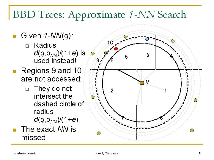
BBD Trees (cont. ) n Exact k-NN(q) search is obtained as follows q q q n Approximate k-NN(q): q n Find the leaf containing the query object Enumerate leaves in the increasing order of distance from q and maintain the k closest objects. Stop when the distance of next leaf is greater than d(q, ok)/(1+e). Distances from q to retrieved objects are at most 1+e times larger than that of the k-th actual nearest neighbor of q. Similarity Search: Part I, Chapter 2 76

BBD Trees: Exact 1 -NN Search n Given 1 -NN(q): 10 9 5 8 3 4 q 2 1 7 Similarity Search: Part I, Chapter 2 6 77

BBD Trees: Approximate 1 -NN Search n Given 1 -NN(q): q n 10 9 5 8 Regions 9 and 10 are not accessed: q n Radius d(q, o. NN)/(1+e) is used instead! They do not intersect the dashed circle of radius d(q, o. NN)/(1+e). 3 4 q 2 1 7 6 The exact NN is missed! Similarity Search: Part I, Chapter 2 78

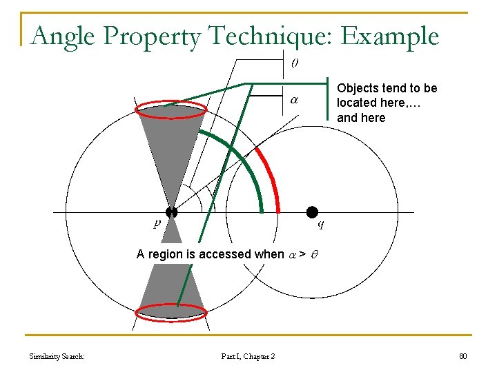
Angle Property Technique n Observed (non-intuitive) properties in high dimensional vector spaces: q Objects tend to have the same distance. n q Parent and child regions have very close radii. n q All regions intersect one each other. The angle formed by a query point, the centre of a ball region, and any data object is close to 90 degrees. n n Therefore they tend to be distributed on the surface of ball regions. The higher the dimensionality, the closer to 90 degrees. These properties can be exploited for approximate similarity search. Similarity Search: Part I, Chapter 2 79

Angle Property Technique: Example Objects tend to be located here, … and here A region is accessed when a > q Similarity Search: Part I, Chapter 2 80

Clustering for Indexing (Clindex) n n Performs approximate similarity search in vector spaces exploiting clustering techniques. The dataset is partitioned into clusters of similar objects: q Each cluster is represented by a separate file sequentially stored on the disk. Similarity Search: Part I, Chapter 2 81

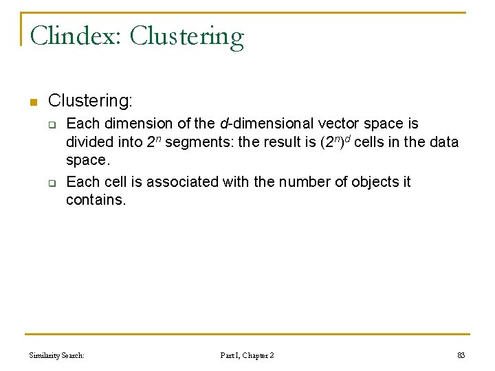
Clindex: Approximate Search n Approximate similarity search: q q n n Seeks for the cluster containing (or the cluster closest to) the query object. Sorts the objects in the cluster according to the distance to the query. The search is approximate since qualifying objects can belong to other (non-accessed) clusters. More clusters can be accessed to improve precision. Similarity Search: Part I, Chapter 2 82

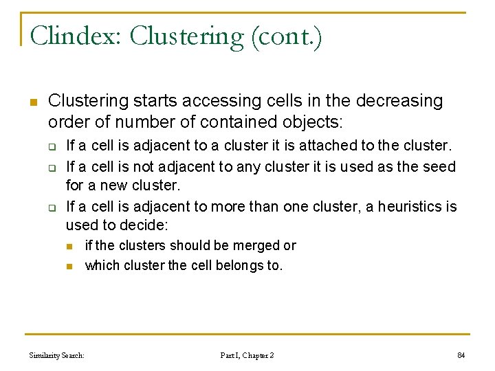
Clindex: Clustering n Clustering: q q Each dimension of the d-dimensional vector space is divided into 2 n segments: the result is (2 n)d cells in the data space. Each cell is associated with the number of objects it contains. Similarity Search: Part I, Chapter 2 83

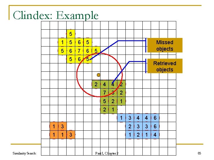
Clindex: Clustering (cont. ) n Clustering starts accessing cells in the decreasing order of number of contained objects: q q q If a cell is adjacent to a cluster it is attached to the cluster. If a cell is not adjacent to any cluster it is used as the seed for a new cluster. If a cell is adjacent to more than one cluster, a heuristics is used to decide: n n Similarity Search: if the clusters should be merged or which cluster the cell belongs to. Part I, Chapter 2 84

Clindex: Example 5 1 5 6 5 5 6 7 6 5 Missed objects 5 Retrieved objects 2 4 4 2 7 3 2 5 2 1 1 Similarity Search: 1 3 1 1 3 Part I, Chapter 2 3 4 4 6 2 3 3 6 1 2 1 4 85

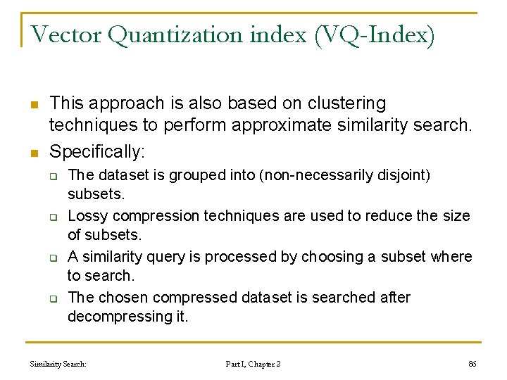
Vector Quantization index (VQ-Index) n n This approach is also based on clustering techniques to perform approximate similarity search. Specifically: q q The dataset is grouped into (non-necessarily disjoint) subsets. Lossy compression techniques are used to reduce the size of subsets. A similarity query is processed by choosing a subset where to search. The chosen compressed dataset is searched after decompressing it. Similarity Search: Part I, Chapter 2 86

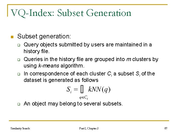
VQ-Index: Subset Generation n Subset generation: q q Query objects submitted by users are maintained in a history file. Queries in the history file are grouped into m clusters by using k-means algorithm. In correspondence of each cluster Ci a subset Si of the dataset is generated as follows An object may belong to several subsets. Similarity Search: Part I, Chapter 2 87

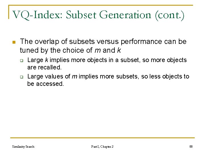
VQ-Index: Subset Generation (cont. ) n The overlap of subsets versus performance can be tuned by the choice of m and k q q Large k implies more objects in a subset, so more objects are recalled. Large values of m implies more subsets, so less objects to be accessed. Similarity Search: Part I, Chapter 2 88

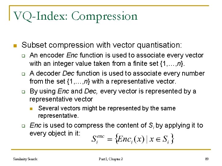
VQ-Index: Compression n Subset compression with vector quantisation: q q q An encoder Enc function is used to associate every vector with an integer value taken from a finite set {1, …, n}. A decoder Dec function is used to associate every number from the set {1, …, n} with a representative vector. By using Enc and Dec, every vector is represented by a representative vector n q Several vectors might be represented by the same representative. Enc is used to compress the content of Si by applying it to every object in it: Similarity Search: Part I, Chapter 2 89

VQ-Index: Approximate Search n Approximate search: q q q Given a query q: The cluster Ci closest to the query is first located. An approximation of Si is reconstructed, by applying the decoder function Deci. The approximation of Si is searched for qualifying objects. Approximation occurs at two stages: n n Similarity Search: Qualifying objects may be included in other subsets, in addition to Si. The reconstructed approximation of Si may contain vectors which differ from the original ones. Part I, Chapter 2 90

Buoy Indexing n n Dataset is partitioned in disjoint clusters. A cluster is represented by a representative element – the buoy. Clusters are bounded by a ball region having the buoy as center and the distance of the buoy to the farthest element of the cluster as the radius. This approach can be used in pure metric spaces. Similarity Search: Part I, Chapter 2 91

Buoy Indexing: Similarity Search n Given an exact k-NN query, clusters are accessed in the increasing distance to their buoys, until current result-set cannot be improved. q That is, until d(q, ok) + ri < d(q, pi) n n pi is the buoy, ri is the radius An approximate k-NN query can be processed by stopping when q q either previous exact condition is true, or a specified ratio f of clusters has been accessed. Similarity Search: Part I, Chapter 2 92

Hierarchical Decomposition of Metric Spaces n In addition to previous ones, there are other methods that were appositively designed to q q n Work on generic metric spaces Organize large collections of data They exploit the hierarchical decomposition of metric spaces. Similarity Search: Part I, Chapter 2 93

Hierarchical Decomposition of Metric Spaces (cont. ) n These will be discussed in details later on: q Relative error approximation n q Relative error on distances of the approximate result is bounded. Good fraction approximation n Similarity Search: Retrieves k objects from a specified fraction of the objects closest to the query. Part I, Chapter 2 94

Hierarchical Decomposition of Metric Spaces (cont. ) n These will be discussed in details later on: q Small chance improvement approximation n q Proximity based approximation n q Stops when chances of improving current result are low. Discards regions with small probability of containing qualifying objects. PAC (Probably Approximately Correct) nearest neighbor search n Similarity Search: Relative error on distances is bounded with a probability specified. Part I, Chapter 2 95