Similarity Flooding A Versatile Graph Matching Algorithm by

Similarity Flooding A Versatile Graph Matching Algorithm by Sergey Melnik, Hector Garcia-Molina, Erhard Rahm 1 Similarity Flooding SDBI – Winter 2001 Yishai Beeri

Introduction & Motivation • Goal: matching elements of related, complex objects • Matching elements of two data schemes • Matching elements of two data instances • Many conceivable uses for object matching • Looking for a generic algorithm with wide applicability 2 Similarity Flooding SDBI – Winter 2001 Yishai Beeri

Applications • Comparing data schemes: – Items from different shopping sites – Merger between two corporations – Preparation of data for data warehousing and analyzing processes • Comparing data instances: – Bio-informatics – Collaboration: allowing multiple users to edit a program / system 3 Similarity Flooding SDBI – Winter 2001 Yishai Beeri

Existing Approaches • Comparing SQL: can use type information • Comparing XML: can use hierarchy Requires domain-specific knowledge and coding Solution: • Generic algorithm that is agnostic to domain • Structural model – relies on structural similarities to find a matching 4 Similarity Flooding SDBI – Winter 2001 Yishai Beeri

Part I: Algorithm Framework General Discussion of Algorithm Input, Output, and Main Components 5 Similarity Flooding SDBI – Winter 2001 Yishai Beeri

Algorithm Framework • Input: two objects to match • Representation of objects as graphs: G 1=(V 1, E 1), G 2=(V 2, E 2) • Matching between graphs gives mapping: V 1 x. V 2 • Filtering of mapping to obtain meaningful match • Output: mapping between elements of input objects Human verification sometimes required 6 Similarity Flooding SDBI – Winter 2001 Yishai Beeri

Input Graph Mapping Filtering • Input are two objects to be matched • Match will be between sub-elements of the two objects • Match of sub-elements will be scored. High scores indicate a strong similarity • Assumption: Objects can be represented as graphs 7 Similarity Flooding SDBI – Winter 2001 Yishai Beeri

Input Graph Mapping Filtering • Represent objects as directed, labeled graphs • Choose any sensible graph representation (this is domain-specific) that maintains structural information • Structural information in graphs will be used for mapping. • Intuition: similar elements have similar neighbors G 1 = (V 1, E 1), G 2 = (V 2, E 2) 8 Similarity Flooding SDBI – Winter 2001 Yishai Beeri

Input Graph Mapping Filtering • We want a mapping : V 1 x. V 2 • Convenient to normalize such that 0 (v, u) 1 • Begin with initial mapping function: – Null function: (v, u) : = 1 for all v in V 1, u in V 2 – String Matching function – Other domain-specific function • Perform an iterative fixpoint calculation. Each iteration floods the similarity value (v, u) to the neighbors of v and u 9 Similarity Flooding SDBI – Winter 2001 Yishai Beeri

Input Graph Mapping Filtering • We have a mapping : V 1 x. V 2 • We are usually not interested in all pairs V 1 x. V 2 • Applying filtering functions yields a partial mapping: – Threshold (only when (v, u) > some constant) – Wedding (each v mapped to only one u and vice versa) • Result is a useful mapping that matches elements of V 1 with elements of V 2 10 Similarity Flooding SDBI – Winter 2001 Yishai Beeri

Part II: An Example - Relational Schemas An Example Employing the Algorithm to Match Two Simple Relational Schemas 11 Similarity Flooding SDBI – Winter 2001 Yishai Beeri

Example: Relational Schemas • Scenario: two relational schemas that describe similar or same data • Goal: match elements of two given relational schemas • Input: SQL statements for creating each scheme • Desired output: a meaningful mapping between the elements of the two schemas 12 Similarity Flooding SDBI – Winter 2001 Yishai Beeri

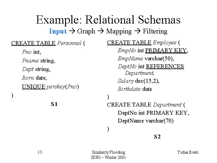
Example: Relational Schemas Input Graph Mapping Filtering CREATE TABLE Personnel ( Pno int, Pname string, Dept string, Born date, UNIQUE perskey(Pno) ) S 1 13 CREATE TABLE Employee ( Emp. No int PRIMARY KEY, Emp. Name varchar(50), Dept. No int REFERENCES Department, Salary dec(15, 2), Birthdate ) CREATE TABLE Department ( Dept. No int PRIMARY KEY, Dept. Name varchar(70) ) S 2 Similarity Flooding SDBI – Winter 2001 Yishai Beeri

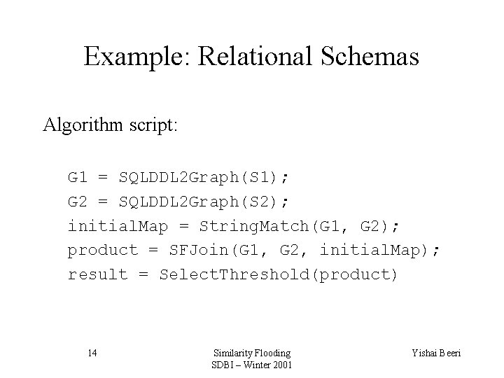
Example: Relational Schemas Algorithm script: G 1 = SQLDDL 2 Graph(S 1); G 2 = SQLDDL 2 Graph(S 2); initial. Map = String. Match(G 1, G 2); product = SFJoin(G 1, G 2, initial. Map); result = Select. Threshold(product) 14 Similarity Flooding SDBI – Winter 2001 Yishai Beeri

Example: Relational Schemas Input Graph Mapping Filtering • Any graph representation of schemas can be chosen • Representation should maintain as much information as possible, in particular structural information • Example uses Open Information Model (OIM) – based graph representation 15 Similarity Flooding SDBI – Winter 2001 Yishai Beeri

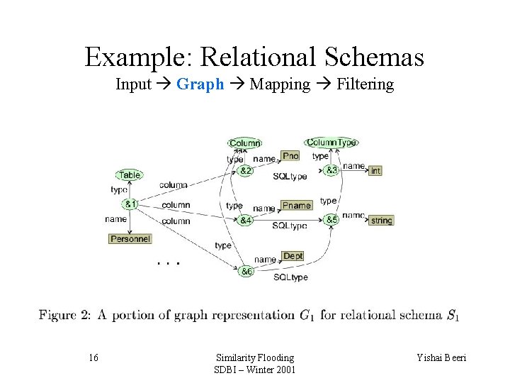
Example: Relational Schemas Input Graph Mapping Filtering 16 Similarity Flooding SDBI – Winter 2001 Yishai Beeri

Example: Relational Schemas Input Graph Mapping Filtering • Calculate initial mapping to improve performance • Initial mapping can apply domain knowledge • In this example: String. Match is used: – Compares common prefixes and suffixes of literals – Assumes elements with similar names have similar meaning – Applies on all elements – including elements that are created by the graph representation (e. g. ‘type’) • Initial mapping still far from satisfactory 17 Similarity Flooding SDBI – Winter 2001 Yishai Beeri

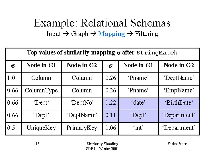
Example: Relational Schemas Input Graph Mapping Filtering Top values of similarity mapping after String. Match Node in G 1 Node in G 2 1. 0 Column 0. 26 ‘Pname’ ‘Dept. Name’ 0. 66 Column. Type Column 0. 26 ‘Pname’ ‘Emp. Name’ 0. 66 ‘Dept’ ‘Dept. No’ 0. 22 ‘date’ ‘Birth. Date’ 0. 66 ‘Dept’ ‘Dept. Name’ 0. 11 ‘Dept’ ‘Department’ 0. 5 Unique. Key Primary. Key 0. 06 ‘int’ ‘Department’ 18 Similarity Flooding SDBI – Winter 2001 Yishai Beeri

Example: Relational Schemas Input Graph Mapping Filtering • Next step: similarity flooding (SFJoin) • Initial similarity values taken from initial mapping • In each iteration similarity of two elements affects the similarity of their respective neighbors (e. g. similarity of type names such as ‘string’ adds to similarity of columns from the same type) • Iterate until similarity values are stable 19 Similarity Flooding SDBI – Winter 2001 Yishai Beeri

Example: Relational Schemas Input Graph Mapping Filtering • After fixpoint calculation, the mapping is filtered to provide a meaningful mapping • The filter operator Select. Threshold removes node pairs for which (u, v) < some constant • In this example, the mapping product contained 211 node pairs with positive similarities, which were filtered to a total of 12 node pairs 20 Similarity Flooding SDBI – Winter 2001 Yishai Beeri

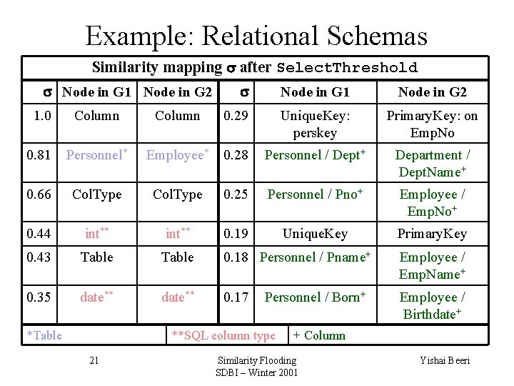
Example: Relational Schemas Similarity mapping after Select. Threshold Node in G 1 Node in G 2 1. 0 Column 0. 29 Unique. Key: perskey Primary. Key: on Emp. No 0. 81 Personnel* Employee* 0. 28 Personnel / Dept+ Department / Dept. Name+ 0. 66 Col. Type 0. 25 Personnel / Pno+ Employee / Emp. No+ 0. 44 int** 0. 19 Unique. Key Primary. Key 0. 43 Table 0. 18 Personnel / Pname+ Employee / Emp. Name+ 0. 35 date** 0. 17 Employee / Birthdate+ *Table Personnel / Born+ **SQL column type 21 + Column Similarity Flooding SDBI – Winter 2001 Yishai Beeri

Example: Relational Schemas Summary of example: • Good results without domain-specific knowledge • Graph representation may vary • Similarity flooding results need to be filtered 22 Similarity Flooding SDBI – Winter 2001 Yishai Beeri

Part III: Similarity Flooding Calculation Details of the Similarity Flooding Calculation Algorithm 23 Similarity Flooding SDBI – Winter 2001 Yishai Beeri

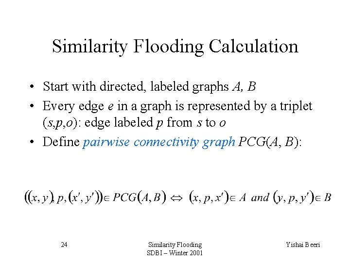
Similarity Flooding Calculation • Start with directed, labeled graphs A, B • Every edge e in a graph is represented by a triplet (s, p, o): edge labeled p from s to o • Define pairwise connectivity graph PCG(A, B): 24 Similarity Flooding SDBI – Winter 2001 Yishai Beeri

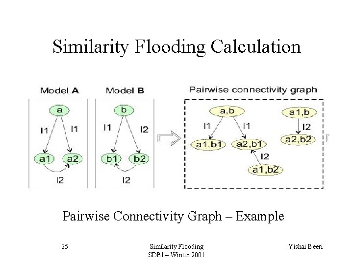
Similarity Flooding Calculation Pairwise Connectivity Graph – Example 25 Similarity Flooding SDBI – Winter 2001 Yishai Beeri

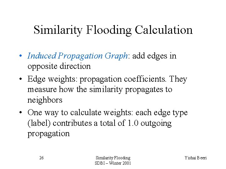
Similarity Flooding Calculation • Induced Propagation Graph: add edges in opposite direction • Edge weights: propagation coefficients. They measure how the similarity propagates to neighbors • One way to calculate weights: each edge type (label) contributes a total of 1. 0 outgoing propagation 26 Similarity Flooding SDBI – Winter 2001 Yishai Beeri

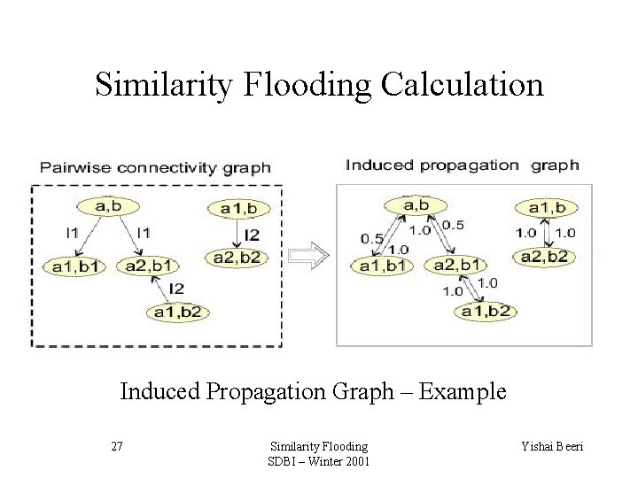
Similarity Flooding Calculation Induced Propagation Graph – Example 27 Similarity Flooding SDBI – Winter 2001 Yishai Beeri

Similarity Flooding Calculation • Similarity measure (x, y) 0 for all x A and b B. We also call a “mapping” • Iterative computation of , with propagation in each iteration • i is the mapping after the i’th iteration • 0 is the initial mapping • Each iteration computes i based on i-1 and the propagation graph • Stop when a stable mapping is reached 28 Similarity Flooding SDBI – Winter 2001 Yishai Beeri

Similarity Flooding Calculation Propagation from i for similarity of x and y is the sum of all similarities from neighbors, each multiplied by the propagation coefficients 29 Similarity Flooding SDBI – Winter 2001 Yishai Beeri

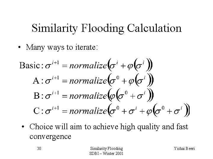
Similarity Flooding Calculation • Many ways to iterate: • Choice will aim to achieve high quality and fast convergence 30 Similarity Flooding SDBI – Winter 2001 Yishai Beeri

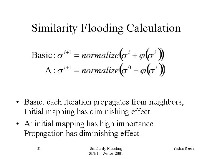
Similarity Flooding Calculation • Basic: each iteration propagates from neighbors; Initial mapping has diminishing effect • A: initial mapping has high importance. Propagation has diminishing effect 31 Similarity Flooding SDBI – Winter 2001 Yishai Beeri

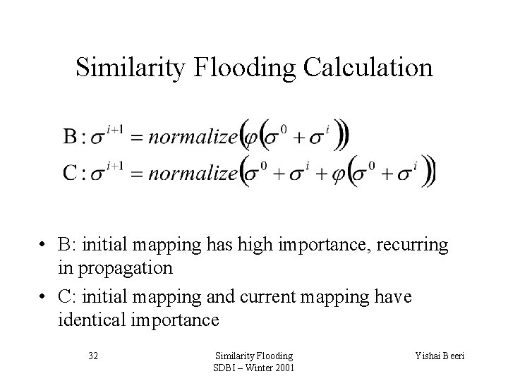
Similarity Flooding Calculation • B: initial mapping has high importance, recurring in propagation • C: initial mapping and current mapping have identical importance 32 Similarity Flooding SDBI – Winter 2001 Yishai Beeri

Part IV: Filtering Overview of Various Approaches to Filtering of SF Mapping 33 Similarity Flooding SDBI – Winter 2001 Yishai Beeri

Filtering • Result of iterations is a mapping between all pairs in V 1 and V 2. We usually want much less information! • Filtering will remove pairs, leaving us with only the interesting ones • There are many ways to filter. Filter choice is domain-specific 34 Similarity Flooding SDBI – Winter 2001 Yishai Beeri

Filtering Possible filtering directions: • Remove uninteresting pairs according to domainspecific knowledge (e. g. ‘column’, ‘table’, ‘string’ from SQL matches) and typing information. • Cardinality considerations: do we want a 1: 1 mapping? A n: m mapping? • Threshold: remove matches with low scores 35 Similarity Flooding SDBI – Winter 2001 Yishai Beeri

Filtering: Cardinality-based filters can use techniques from bilateral graph (“marriage”) problems: • Stable marriage • Assignment problem: max. of (x, y) • Maximum mapping: max. number of 1: 1 matches • Maximal mapping: not contained in other mapping • Perfect/Complete: all are “married” All the above give [0, 1]: [0, 1] (monogamous) matches, and can be found in polynomial time 36 Similarity Flooding SDBI – Winter 2001 Yishai Beeri

Filtering: Relative Similarity • (x, y) is the absolute similarity of x and y • We can also define a relative similarity: • Relative similarity is directed. The reverse direction is defined in an analogue manner • Bipartite graph methods can also handle directed graphs 37 Similarity Flooding SDBI – Winter 2001 Yishai Beeri

Filtering: Threshold • Threshold can be applied to absolute or relative similarities • A useful example: threshold of trel=1. 0 gives a perfectionist egalitarian polygamy – e. g. no man/woman is willing to accept any but the best match 38 Similarity Flooding SDBI – Winter 2001 Yishai Beeri

Part V: Examples of Algorithm Application to Various Problems 39 Similarity Flooding SDBI – Winter 2001 Yishai Beeri

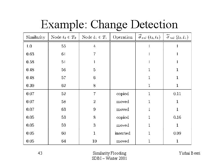
Example: Change Detection • Goal: change detection in two labeled trees • Original tree T 1 was changed to give T 2: – Node names were replaced – Subtrees were copied and moved – New node was inserted • We want the best match for every node of T 2 – Cardinality constraint: [0, n] – [1, 1] 40 Similarity Flooding SDBI – Winter 2001 Yishai Beeri

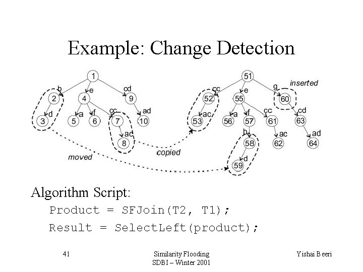
Example: Change Detection Algorithm Script: Product = SFJoin(T 2, T 1); Result = Select. Left(product); 41 Similarity Flooding SDBI – Winter 2001 Yishai Beeri

Example: Change Detection • No initial mapping • Select. Left operator selects best absolute match for each element in left argument • Results can also provide hints on type of change that was performed! 42 Similarity Flooding SDBI – Winter 2001 Yishai Beeri

Example: Change Detection 43 Similarity Flooding SDBI – Winter 2001 Yishai Beeri

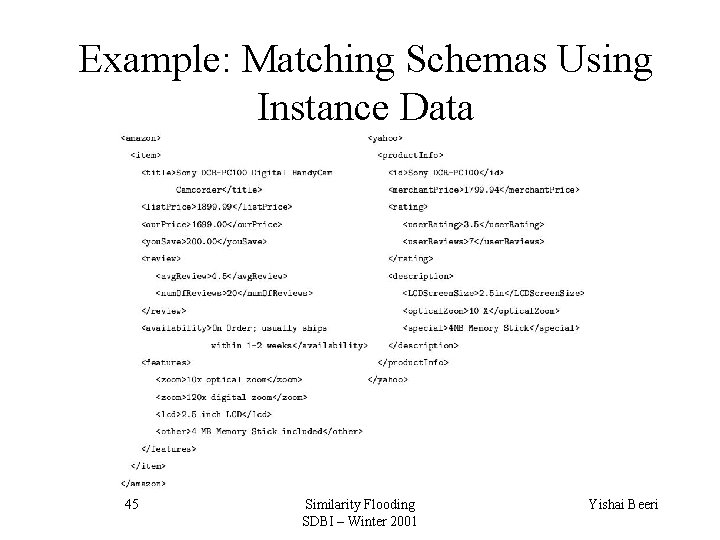
Example: Matching Schemas Using Instance Data • Goal: match two XML Schemas using instance data • Two XML product descriptions from two shopping websites • We want to use the instance data to match the XML schemas 44 Similarity Flooding SDBI – Winter 2001 Yishai Beeri

Example: Matching Schemas Using Instance Data 45 Similarity Flooding SDBI – Winter 2001 Yishai Beeri

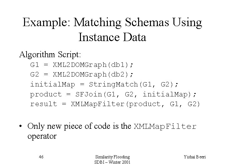
Example: Matching Schemas Using Instance Data Algorithm Script: G 1 = XML 2 DOMGraph(db 1); G 2 = XML 2 DOMGraph(db 2); initial. Map = String. Match(G 1, G 2); product = SFJoin(G 1, G 2, initial. Map); result = XMLMap. Filter(product, G 1, G 2) • Only new piece of code is the XMLMap. Filter operator 46 Similarity Flooding SDBI – Winter 2001 Yishai Beeri

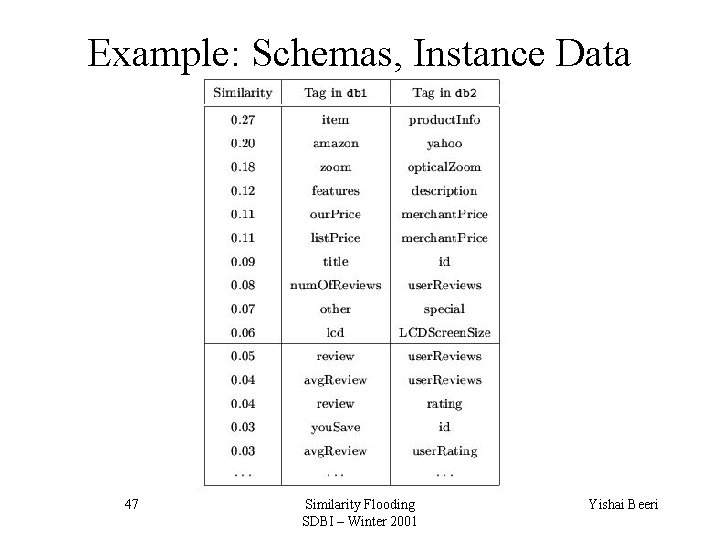
Example: Schemas, Instance Data 47 Similarity Flooding SDBI – Winter 2001 Yishai Beeri

Part VI: Analysis Match Quality, Algorithm Complexity, Convergence and Limitations 48 Similarity Flooding SDBI – Winter 2001 Yishai Beeri

Match Quality • Assessing match quality is difficult • Human verification and tuning of matching is often required • A useful metric would be to measure the amount of human work required to reach the perfect match • Recall: how many good matches did we show? • Precision: how many of the matches we show are good? 49 Similarity Flooding SDBI – Winter 2001 Yishai Beeri

Convergence • Fixpoint iterations are an eigenvector computation for the matrix that corresponds to the propagation graph • Computation converges iff graph is strongly connected • To achieve this we use dampening: use 0 in the fixpoint formula, where 0(x, y) > 0 for all x, y • Convergence rate depends on spectral radius of the matrix, and can be improved by high dampening values 50 Similarity Flooding SDBI – Winter 2001 Yishai Beeri

Convergence • In many cases we are only interested in order of map pairs, and not absolute values of . • The order usually stabilizes before the actual values do 51 Similarity Flooding SDBI – Winter 2001 Yishai Beeri

Complexity • Usually 5 -30 iterations • Each iteration is O(|E|) (edges in propagation graph) • |E| = O(|E 1| • |E 2|) • |E 1| = O(|V 1|2) – if G 1 is highly connected • |E 2| = O(|V 2|2) – if G 2 is highly connected • Worst case of each iteration is O(|V 1|2 • |V 2|2) • Average case of each iteration is O(|V 1| • |V 2|) 52 Similarity Flooding SDBI – Winter 2001 Yishai Beeri

Limitations • Algorithm requires representation as directed, labeled graph – Degrades when edges are unlabeled or undirected – Degrades when labeling is more uniform • Assumes structural adjacency contributes to similarity – Will not work for matching HTML • Requires matched objects to be of same type and with same graph representation 53 Similarity Flooding SDBI – Winter 2001 Yishai Beeri

Limitations • Algorithm cannot utilize order and aggregation information (e. g. for XML) – Order: the order of sub-elements within an element – Aggregation: an element containing an “array” of subelements 54 Similarity Flooding SDBI – Winter 2001 Yishai Beeri

Part VII: Variability and Applications Discussion of Algorithm Variability Areas and Possible Applications 55 Similarity Flooding SDBI – Winter 2001 Yishai Beeri

Variability in Algorithm • • • Graph representation of input objects Calculation of propagation coefficients Initial mapping function Iteration formula Filtering function 56 Similarity Flooding SDBI – Winter 2001 Yishai Beeri

Graph Representation • Graph representation of input objects is arbitrary; sub-elements can be modeled as nodes, edges, or both. • On one hand: – Richer graph captures more structure information – Type information about sub-elements can be modeled • On the other hand: – Larger graphs mean longer computation – Rich graph often implies more uniform labeling 57 Similarity Flooding SDBI – Winter 2001 Yishai Beeri

Propagation Coefficients • Propagation coefficients can be calculated in many ways: – Sum of all outgoing edges is 1. 0 – Equal weigh (1. 0) for all edges – Sum of all outgoing edges of label ‘p’ is 1. 0 – Sum of all incoming edges is 1. 0 – Label-specific weight allocation – Etc. 58 Similarity Flooding SDBI – Winter 2001 Yishai Beeri

Initial Mapping Function • Initial mapping can improve performance and help convergence • Initial mapping function can be naïve, or it can employ domain-specific knowledge 59 Similarity Flooding SDBI – Winter 2001 Yishai Beeri

Iteration Formula • Each iteration calculates i+1 from i , 0, and ( i) • Iteration formula can vary, giving different weight and effect to these components – Example: if initial mapping is good, give higher weight to 0 • Formula affects convergence speed as well as resultant mapping 60 Similarity Flooding SDBI – Winter 2001 Yishai Beeri

Filtering Function • Results of iterations require filtering to become a meaningful mapping • Many approaches to filtering are possible, as discussed • Choice usually stems from graph representation and specific goal. For example: – If graphs contain many type-related nodes, they can be pruned from results – If goal is to detect changes, we want a match for each element of the newer object 61 Similarity Flooding SDBI – Winter 2001 Yishai Beeri

Applications There are many possible applications besides the ones described: • Comparing websites – Old vs. new versions of website – Two websites with information about same subject – Structural information gained from containment and links 62 Similarity Flooding SDBI – Winter 2001 Yishai Beeri

Applications • Natural language processing and speech recognition: – Match given sentence to XML template – Match two text segments that refer to the same subject • Finding self-similarities and related data items by running SFJoin(G, G) • Preparation of data and schemas for data warehousing and data mining – Canonization of data and meta-data 63 Similarity Flooding SDBI – Winter 2001 Yishai Beeri

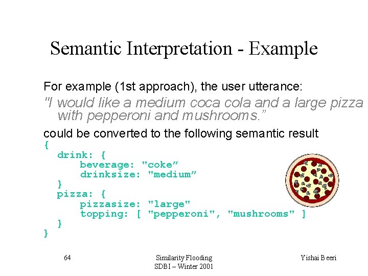
Semantic Interpretation - Example For example (1 st approach), the user utterance: "I would like a medium coca cola and a large pizza with pepperoni and mushrooms. ” could be converted to the following semantic result { } drink: { beverage: "coke” drinksize: "medium” } pizza: { pizzasize: "large" topping: [ "pepperoni", "mushrooms" ] } 64 Similarity Flooding SDBI – Winter 2001 Yishai Beeri

Applications • More… 65 Similarity Flooding SDBI – Winter 2001 Yishai Beeri

Summary • Generic algorithm – with many applications • Relies on structural information captured in graph representation • Domain-specific customizations can improve performance and match quality • Useful but does not deliver 100% exact results; human verification often required 66 Similarity Flooding SDBI – Winter 2001 Yishai Beeri