SIGNAL PROCESSING SOME APPLICATIONS IN SPEECH MUSIC and

SIGNAL PROCESSING: SOME APPLICATIONS IN SPEECH, MUSIC, and IMAGE PROCESSING Richard M. Stern 18 -396 demo January 12, 2009 Department of Electrical and Computer Engineering and School of Computer Science Carnegie Mellon University Pittsburgh, Pennsylvania 15213

What is signal processing? Oppenheim and Schafer’s definition (1999): – [The discipline that is concerned with] the representation, transformation, and manipulation of signals and the information they contain Carnegie Mellon Slide 2 18 -396 Signals and Systems

Why perform signal processing? To understand the content of signals To represent signals in a form that is more insightful to us To transform signals into a form that is more useful to us Carnegie Mellon Slide 3 18 -396 Signals and Systems

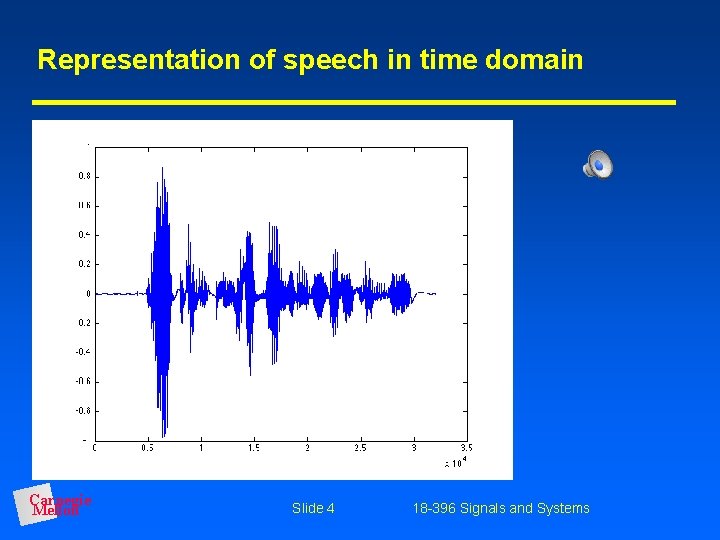
Representation of speech in time domain Carnegie Mellon Slide 4 18 -396 Signals and Systems

Representation of speech in frequency domain Carnegie Mellon Slide 5 18 -396 Signals and Systems

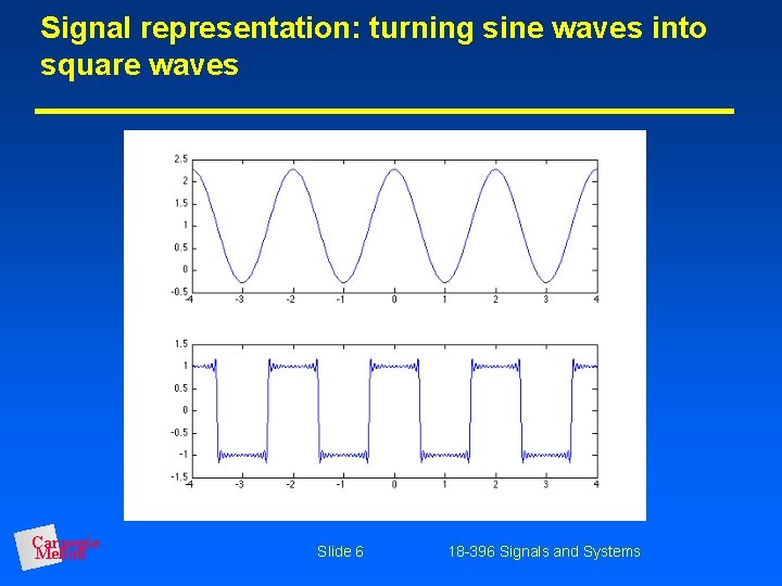
Signal representation: turning sine waves into square waves Carnegie Mellon Slide 6 18 -396 Signals and Systems

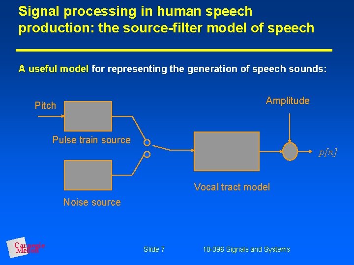
Signal processing in human speech production: the source-filter model of speech A useful model for representing the generation of speech sounds: Amplitude Pitch Pulse train source p[n] Vocal tract model Noise source Carnegie Mellon Slide 7 18 -396 Signals and Systems

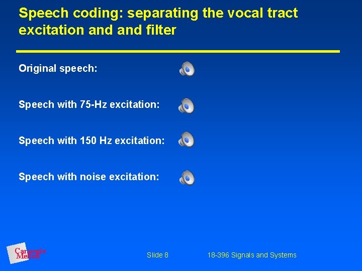
Speech coding: separating the vocal tract excitation and filter Original speech: Speech with 75 -Hz excitation: Speech with 150 Hz excitation: Speech with noise excitation: Carnegie Mellon Slide 8 18 -396 Signals and Systems

Representation and filtering of speech sounds Carnegie Mellon Slide 9 18 -396 Signals and Systems

Linear filtering the waveform y[n] x[n] Filter 1: y[n] = 3. 6 y[n– 1]+5. 0 y[n– 2]– 3. 2 y[n– 3]+. 82 y[n– 4] +. 013 x[n]–. 032 x[n– 1]+. 044 x[n– 2]–. 033 x[n– 3]+. 013 x[n– 4] Filter 2: y[n] = 2. 7 y[n– 1]– 3. 3 y[n– 2]+2. 0 y[n– 3–. 57 y[n– 4] +. 35 x[n]– 1. 3 x[n– 1]+2. 0 x[n– 2]– 1. 3 x[n– 3]+. 35 x[n– 4] Carnegie Mellon Slide 10 18 -396 Signals and Systems

Filter 1 in the time domain Carnegie Mellon Slide 11 18 -396 Signals and Systems

Output of Filter 1 in the frequency domain Original: Lowpass: Carnegie Mellon Slide 12 18 -396 Signals and Systems

Filter 2 in the time domain Carnegie Mellon Slide 13 18 -396 Signals and Systems

Output of Filter 2 in the frequency domain Original: Highpass: Carnegie Mellon Slide 14 18 -396 Signals and Systems

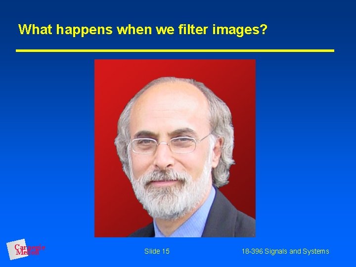
What happens when we filter images? Carnegie Mellon Slide 15 18 -396 Signals and Systems

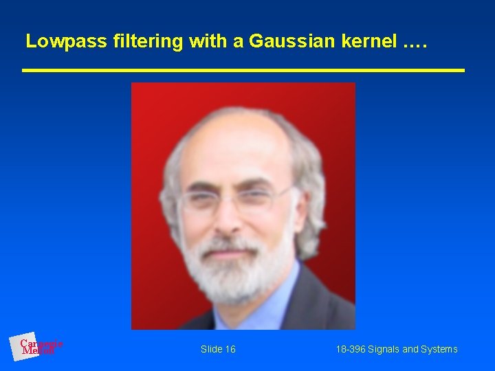
Lowpass filtering with a Gaussian kernel …. Carnegie Mellon Slide 16 18 -396 Signals and Systems

Not enough blur? ? Carnegie Mellon Slide 17 18 -396 Signals and Systems

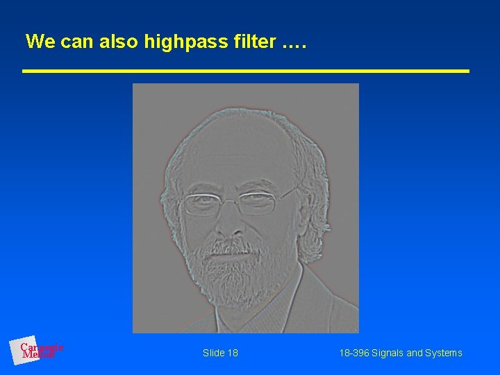
We can also highpass filter …. Carnegie Mellon Slide 18 18 -396 Signals and Systems

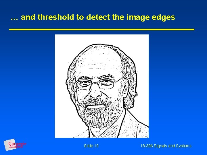
… and threshold to detect the image edges Carnegie Mellon Slide 19 18 -396 Signals and Systems