SIGNAL FLOW GRAPH Outline Introduction to Signal Flow

SIGNAL FLOW GRAPH

Outline • Introduction to Signal Flow Graphs – Definitions – Terminologies • Mason’s Gain Formula – Examples • Signal Flow Graph from Block Diagrams • Examples

Signal Flow Graph (SFG) • Alternative method to block diagram representation, developed by Samuel Jefferson Mason. • Block diagram are adequate for representation but cumbersome. • A signal-flow graph provides the relation between system variables without requiring any reduction procedures.

Fundamentals of Signal Flow Graphs Consider a simple equation below and draw its signal flow graph: The signal flow graph of the equation is shown below;

Important terminology : • Branches : line joining two nodes is called branch. Branch • Dummy Nodes: A branch having one can be added at i/p as well as o/p. Dummy Nodes

Input & output node • Input node: It is node that has only outgoing branches. • Output node: It is a node that has incoming branches. f x 0 x 1 a b c d x 2 x 3 g h x 4 e Input node Out put node

Forward path: • Any path from i/p node to o/p node. Forward path

Loop : • A closed path from a node to the same node is called loop.

Self loop: • A feedback loop that contains of only one node is called self loop. Self loop

Loop gain: The product of all the gains forming a loop Loop gain = A 32 A 23

Path & path gain Path: - A path is a traversal of connected branches in the direction of branch arrow. Path gain: The product of all branch gains while going through the forward path it is called as path gain.

Feedback path or loop : • it is a path to o/p node to i/p node.

Touching loops: • when the loops are having the common node that the loops are called touching loops.

Non touching loops: • when the loops are not having any common node between them that are called as non- touching loops.

Non-touching loops forward paths

Chain Node : • it is a node that has incoming as well as outgoing branches. Chain node

Mason’s Rule (Mason, 1953) • The block diagram reduction technique requires successive application of fundamental relationships in order to arrive at the system transfer function. • On the other hand, Mason’s rule for reducing a signal-flow graph to a single transfer function requires the application of one formula.

Mason’s Rule : • The transfer function, C(s)/R(s), of a system represented by a signal-flow graph is; • Where • • n = number of forward paths. Pi = the i th forward-path gain. ∆ = Determinant of the system ∆i = Determinant of the ith forward path

∆ is called the signal flow graph determinant or characteristic function. Since ∆=0 is the system characteristic equation. ∆ = 1 - (sum of all individual loop gains) + (sum of the products of the gains of all possible two loops that do not touch each other) – (sum of the products of the gains of all possible three loops that do not touch each other) + … and so forth with sums of higher number of non-touching loop gains ∆i = value of Δ for the part of the block diagram that does not touch the i-th forward path (Δi = 1 if there are no non-touching loops to the i-th path. )

Example 1: Apply Mason’s Rule to calculate the transfer function of the system represented by following Signal Flow Graph Therefore, There are three feedback loops Continue……

There are no non-touching loops, therefore ∆ = 1 - (sum of all individual loop gains) Continue……

Eliminate forward path-1 ∆1 = 1 - (sum of all individual loop gains)+. . . ∆1 = 1 Eliminate forward path-2 ∆2 = 1 - (sum of all individual loop gains)+. . . ∆2 = 1 Continue……

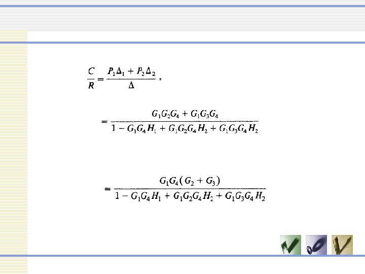
From Block Diagram to Signal-Flow Graph Models • Example 2 R(s) E(s) H 1 X 1 G 1 － － － G 2 X 3 G 4 C(s) H 2 H 3 R(s) 1 E(s) G 1 X 1 G 2 X 2 G 3 －H 1 G 4 X 3 1 C(s) －H 2 －H 3 Continue……

R(s) 1 E(s) G 1 X 1 G 2 －H 3 X 2 G 3 －H 1 G 4 X 3 1 C(s)

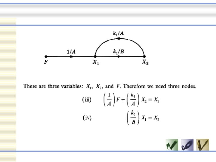
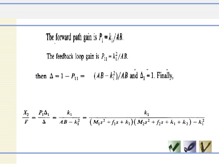
Design example Example 3

Example 4 Continue……

Continue……