SIFTs ScaleSpace From a presentation by Jimmy Huff

SIFT’s Scale-Space From a presentation by Jimmy Huff Modified by Josiah Yoder

Scale-Space Extrema Detection – Get the Points! • Scale-space groups an image into an octave with S levels. • The smoothing is done incrementally such that σ of the S + 1 image in the octave is twice that of the first image.
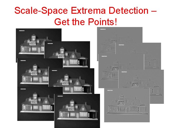
Scale-Space Extrema Detection – Get the Points!
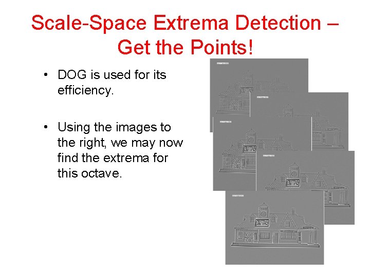
Scale-Space Extrema Detection – Get the Points! • DOG is used for its efficiency. • Using the images to the right, we may now find the extrema for this octave.
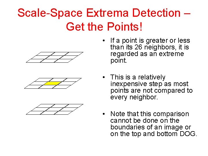
Scale-Space Extrema Detection – Get the Points! • If a point is greater or less than its 26 neighbors, it is regarded as an extreme point. • This is a relatively inexpensive step as most points are not compared to every neighbor. • Note that this comparison cannot be done on the boundaries of an image or on the top and bottom DOG.

Scale-Space Extrema Detection – Get the Points! σ 2σ . . . As sample Each octave points is processed starts are with collected, σ twice the separately. value they are of σ stored of theas previous a three-vector octave and continues to increase. p = (x, y, σ) [σ being scale in this case]
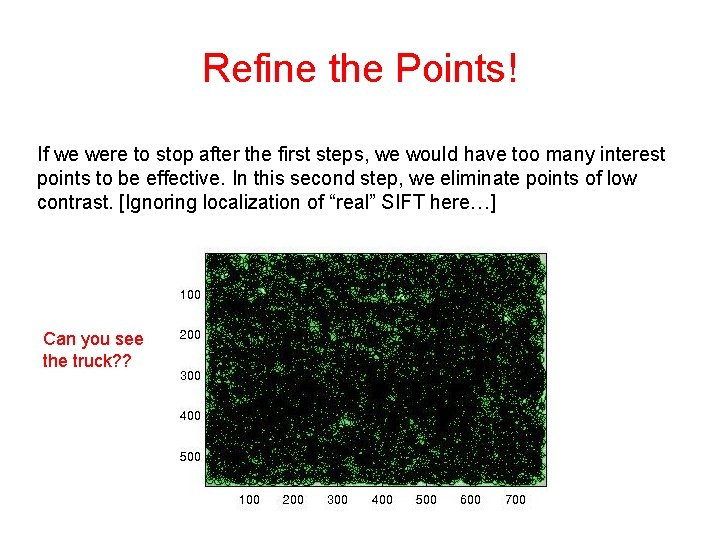
Refine the Points! If we were to stop after the first steps, we would have too many interest points to be effective. In this second step, we eliminate points of low contrast. [Ignoring localization of “real” SIFT here…] Can you see the truck? ?
Refine the Points! Only keep points where DOG > some threshold (e. g. 3% of maximum intensity in original image)
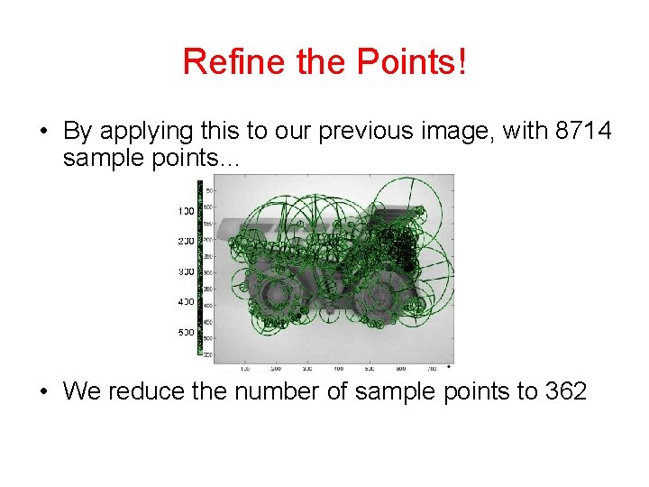
Refine the Points! • By applying this to our previous image, with 8714 sample points… • We reduce the number of sample points to 362

Save for later
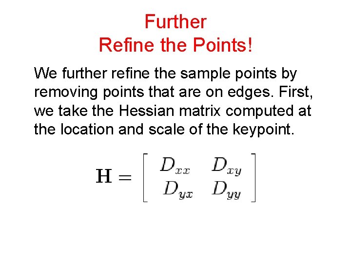
Further Refine the Points! We further refine the sample points by removing points that are on edges. First, we take the Hessian matrix computed at the location and scale of the keypoint.
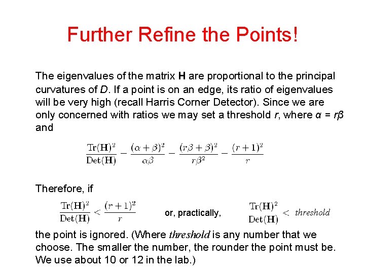
Further Refine the Points! The eigenvalues of the matrix H are proportional to the principal curvatures of D. If a point is on an edge, its ratio of eigenvalues will be very high (recall Harris Corner Detector). Since we are only concerned with ratios we may set a threshold r, where α = rβ and Therefore, if or, practically, threshold the point is ignored. (Where threshold is any number that we choose. The smaller the number, the rounder the point must be. We use about 10 or 12 in the lab. )
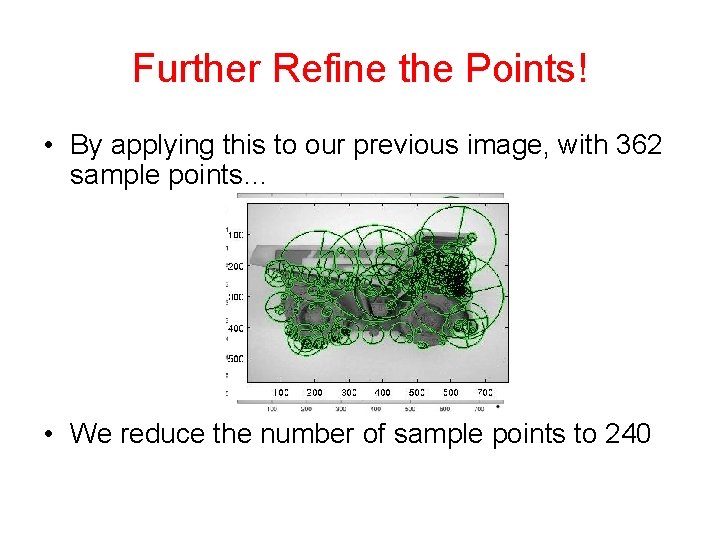
Further Refine the Points! • By applying this to our previous image, with 362 sample points… • We reduce the number of sample points to 240
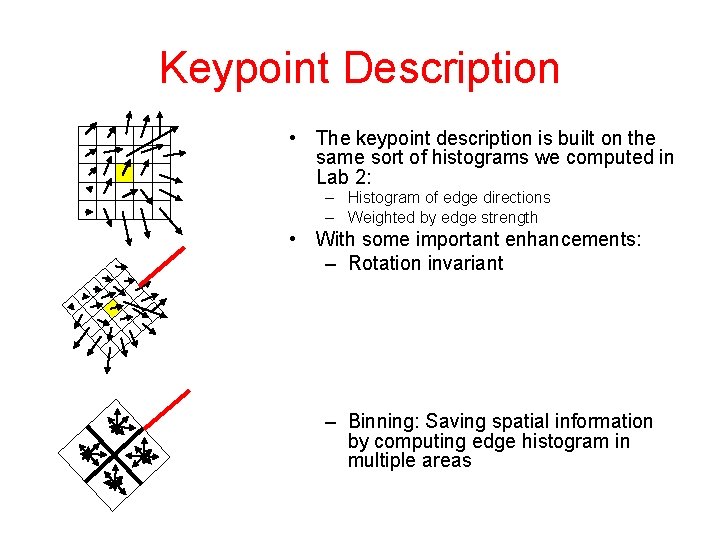
Keypoint Description • The keypoint description is built on the same sort of histograms we computed in Lab 2: – Histogram of edge directions – Weighted by edge strength • With some important enhancements: – Rotation invariant – Binning: Saving spatial information by computing edge histogram in multiple areas
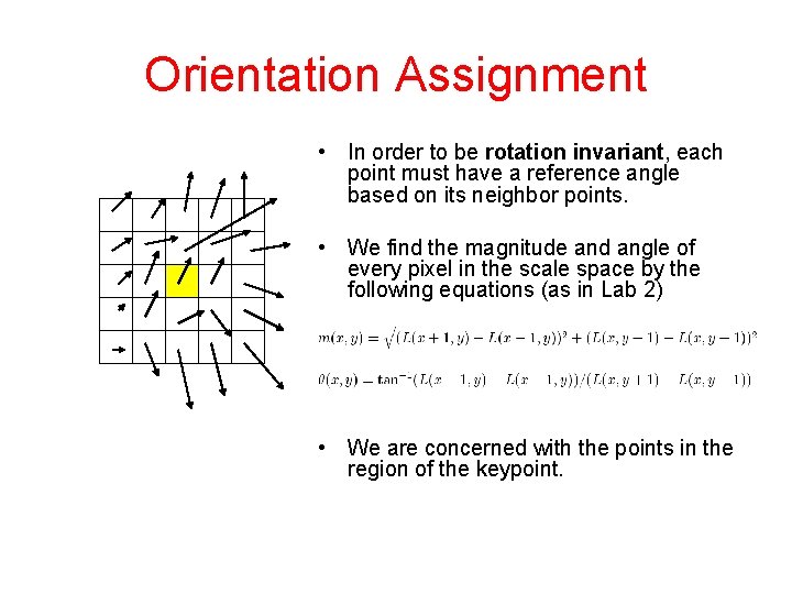
Orientation Assignment • In order to be rotation invariant, each point must have a reference angle based on its neighbor points. • We find the magnitude and angle of every pixel in the scale space by the following equations (as in Lab 2) • We are concerned with the points in the region of the keypoint.
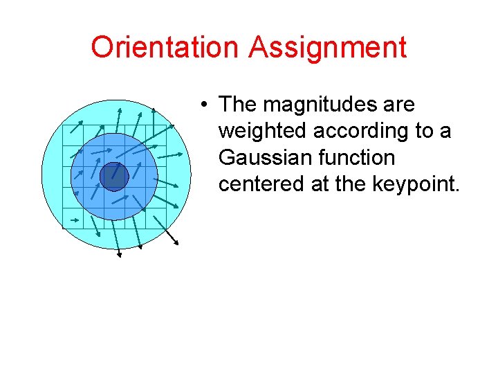
Orientation Assignment • The magnitudes are weighted according to a Gaussian function centered at the keypoint.
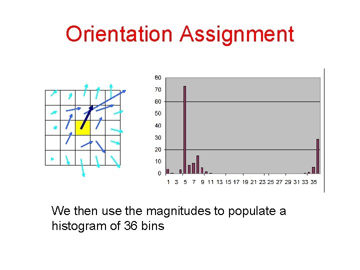
Orientation Assignment We then use the magnitudes to populate a histogram of 36 bins
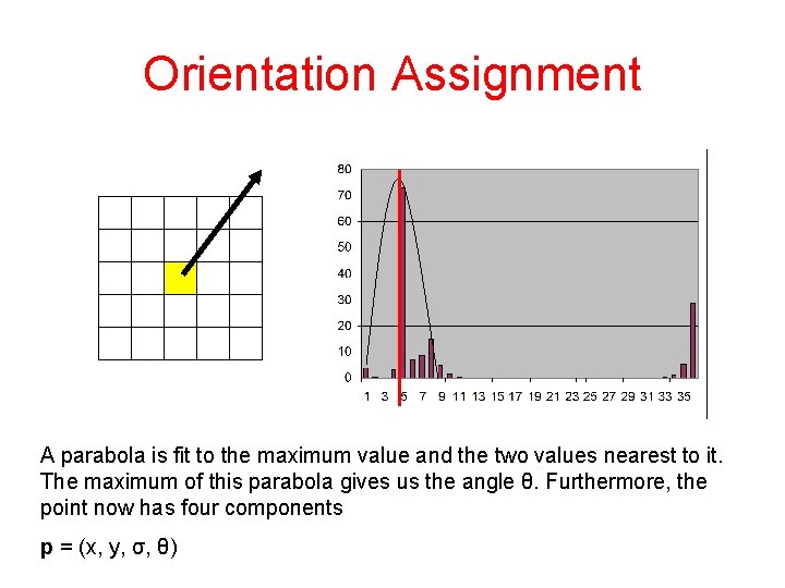
Orientation Assignment A parabola is fit to the maximum value and the two values nearest to it. The maximum of this parabola gives us the angle θ. Furthermore, the point now has four components p = (x, y, σ, θ)
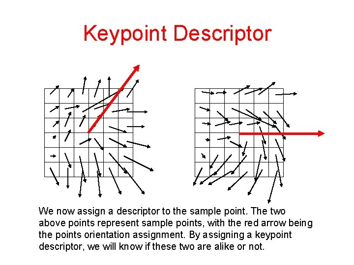
Keypoint Descriptor We now assign a descriptor to the sample point. The two above points represent sample points, with the red arrow being the points orientation assignment. By assigning a keypoint descriptor, we will know if these two are alike or not.
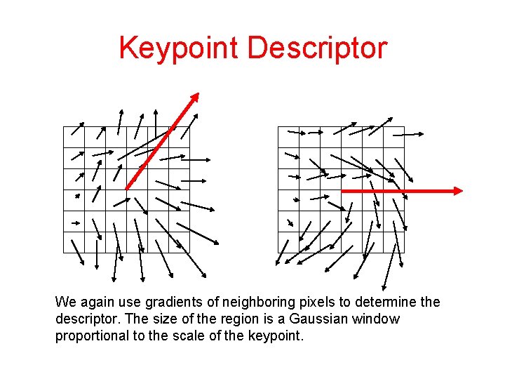
Keypoint Descriptor We again use gradients of neighboring pixels to determine the descriptor. The size of the region is a Gaussian window proportional to the scale of the keypoint.
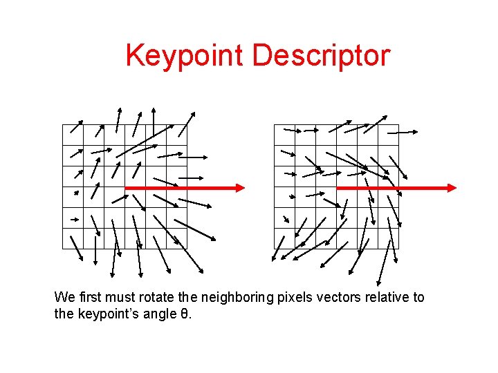
Keypoint Descriptor We first must rotate the neighboring pixels vectors relative to the keypoint’s angle θ.
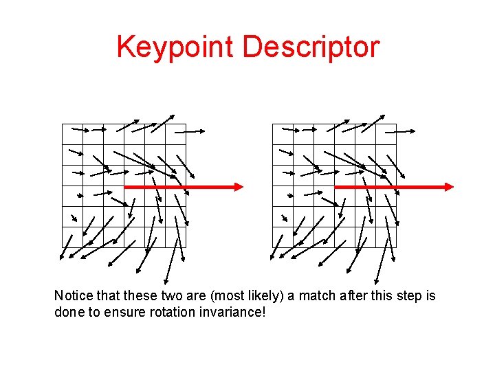
Keypoint Descriptor Notice that these two are (most likely) a match after this step is done to ensure rotation invariance!
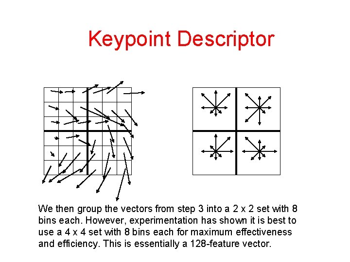
Keypoint Descriptor We then group the vectors from step 3 into a 2 x 2 set with 8 bins each. However, experimentation has shown it is best to use a 4 x 4 set with 8 bins each for maximum effectiveness and efficiency. This is essentially a 128 -feature vector.
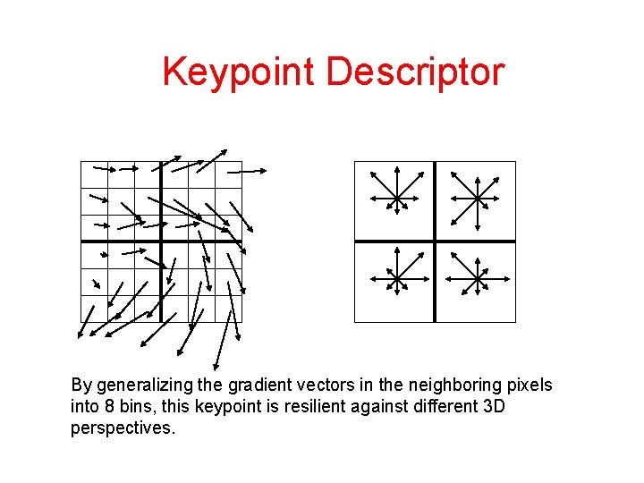
Keypoint Descriptor By generalizing the gradient vectors in the neighboring pixels into 8 bins, this keypoint is resilient against different 3 D perspectives.
Keypoint Descriptor In order to be resilient to differences in illumination, we normalize the entries of the feature vector. This makes the descriptor invariant to changes in contrast or brightness In order to be resilient to non-linear changes in illumination, such as camera saturation, we reduce the effect of large gradient vectors by setting a threshold in the feature vector such that no value is larger than 0. 2. We then re-normalize.
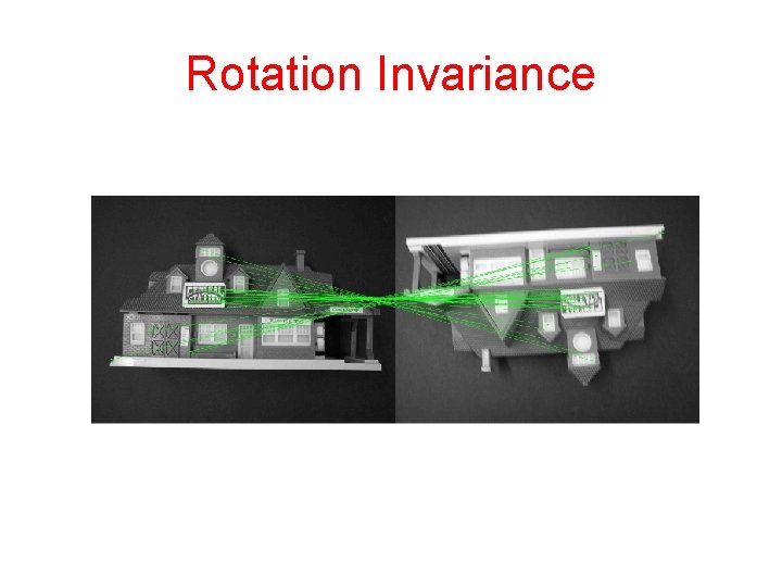
Rotation Invariance
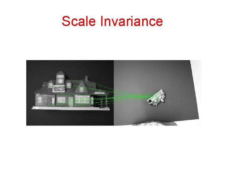
Scale Invariance
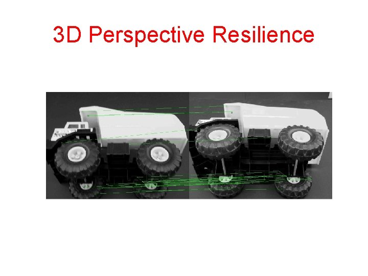
3 D Perspective Resilience
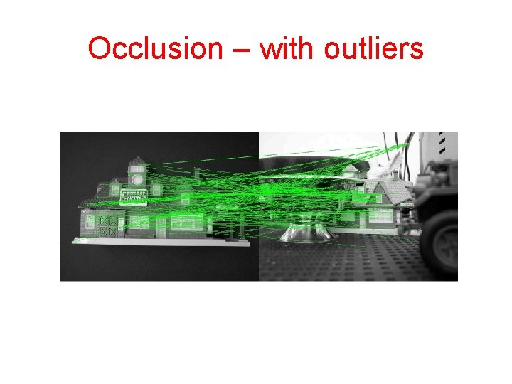
Occlusion – with outliers
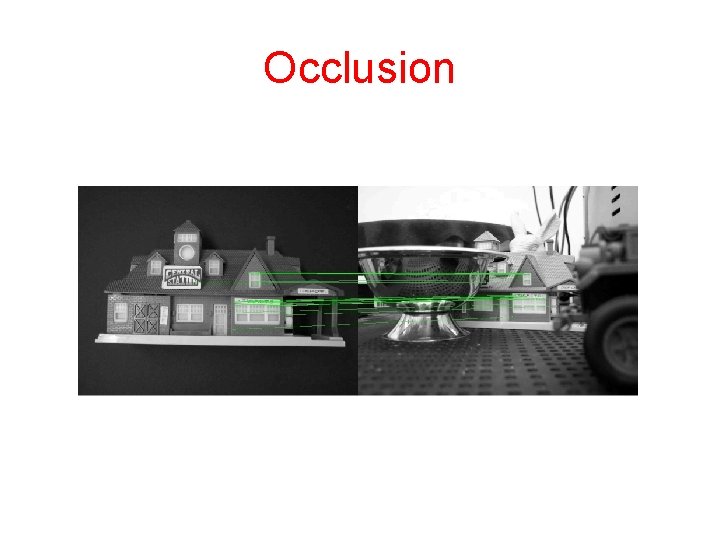
Occlusion
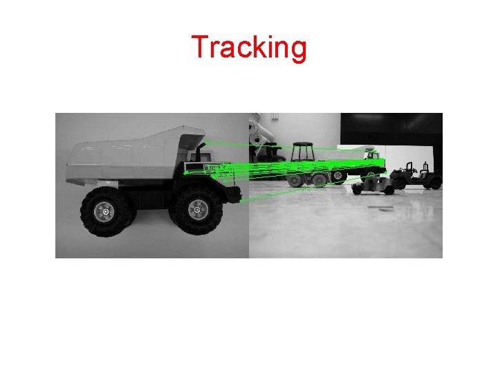
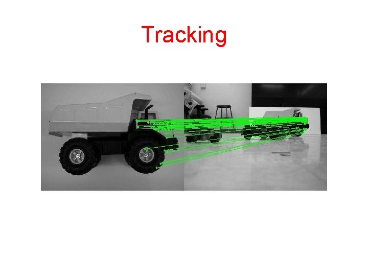
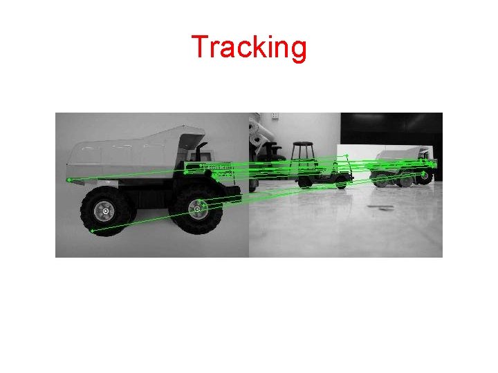
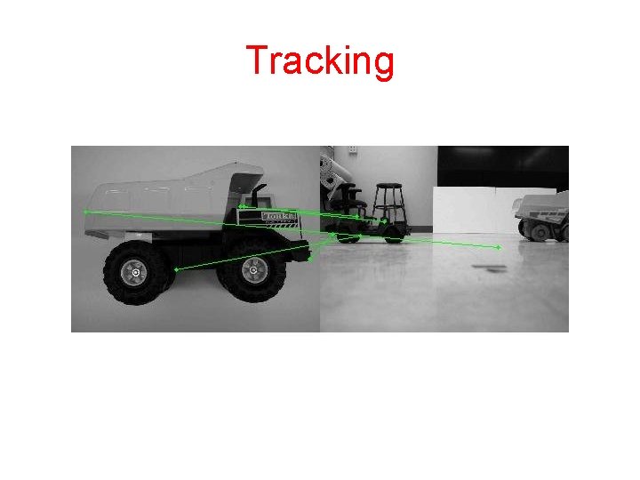
Tracking
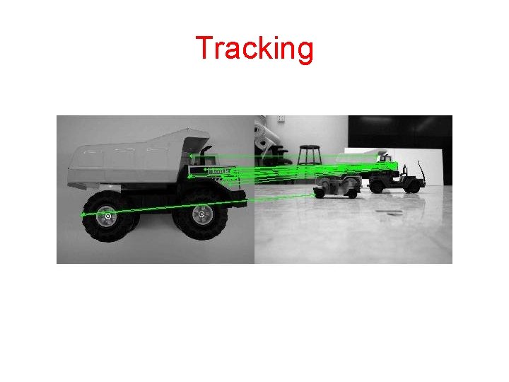
Tracking
Tracking
Tracking
Tracking
- Slides: 35