Shortwave and longwave contributions to global warming under

Shortwave and longwave contributions to global warming under increased CO 2 Aaron Donohoe, University of Washington CLIVAR CONCEPT HEAT Meeting Exeter, September 30, 2015

Energy imbalance and temperature change Unperturbed ASR = OLR Atmospheric Emission Level Solar Perturbation Greenhouse Perturbation ASR=> OLR CO 2 ASR = OLR ASR > OLR

Top of Atmosphere Radiative response to greenhouse and shortwave forcing OLR returns to unperturbed value in 20 years

Proposed solution – Positive SW feedback Absorbed Solar Radiation Outgoing Longwave Radiation Atmospheric Emission Level Unperturbed ADD CO 2 ASR > OLR

Absorbed Solar Radiation Outgoing Longwave Radiation Atmospheric Emission Level CO 2 + Warming + Feedback Proposed solution – Positive SW feedback OLRASR Increases WARMING

Absorbed Solar Radiation Outgoing Longwave Radiation Atmospheric Emission Level OLR = Unperturbed Energy still accumulating Proposed solution – Positive SW feedback WARMING

Absorbed Solar Radiation Outgoing Longwave Radiation Atmospheric Emission Level New Equilibrium OLR = ASR BOTH INCRESED Proposed solution – Positive SW feedback WARMING

Inter-model spread in TOA response The TOA response to greenhouse forcing differs a lot between GCMs • OLR returns to unperturbed values (ΤCROSS) within 5 years for some GCMs and not at all for others (bi-modal) • On average, ΤCROSS = 19 years Ensemble mean
 radiation Energy Change Forcing Feedbacks • C")
Linear Feedback model Top of atmosphere (TOA) radiation Energy Change Forcing Feedbacks • C = heat capacity of climate system. Time dependent – meters of ocean • TS = Global mean surface temperature change • FSW and FLW are the SW and LW radiative forcing (including fast cloud response to radiative forcing – W m-2) • λLW and λSW are the LW and SW feedback parameters. W m-2 K-1 • Given above parameters and TS , we can predict the TOA response

Backing out Forcing and feedbacks from instantaneous 4 XCO 2 increase runs CNRM model • Feedbacks parameters (λLW and λSW) are the slope of –OLR and ASR vs. TS (W m-2 K-1) • Forcing (FSW and FLW) is the intercept (W m-2 ). Includes rapid cloud response to CO 2 (Gregory and Webb)
 –")
Linear Feedback model works The TOA response in each model (and ensemble average) – solid lines– is well replicated by the linear feedback model • What parameters (forcing, feedbacks, heat capacity) set the mean radiative response and its variations across models?

Ensemble average OLR recovery timescale Ensemble average forcing and feedbacks • λLW = -1. 7 W m-2 K-1 • λSW = +0. 6 W m-2 K-1 • FLW = + 6. 1 W m-2 OLR at equilibrium OLR at time = 0 equilibrium temperature change ASR in new equilibrium = TEQ λSW = 4 W m-2 • To come to equilibrium, OLR must go from - FLW = - 6. 1 W m-2 to TEQ λLW = +4 W m-2 • OLR must change by 10 W m-2 to come to equilibrium OLR crosses zero about 60% of the way the equilibrium

Climate model differences in OLR response time CNRM model
: τCROSS = τ")
Sensitivity of τCROSS to feedback parameters If FSW = 0 (simplification): τCROSS = τ ln(-λ LW / λ SW ) τcross is determined by the OLR value demanded in the new equilibrium Set by relative magnitudes of λ LW and λ SW HAS STEEP GRADIENTS IN VICINITY OF λSW=0 Ensemble Average
 transmitted ocean")
Cause of SW positive feedbacks: incident absorbed Reflected cloud H 20 (vapor) transmitted ocean Surface albedo feedback = +0. 26 ± 0. 08 W m-2 K-1 Bony et al. (2006) Reflected surface ice SW Water vapor feedback = +0. 3± 0. 1 W m-2 K-1

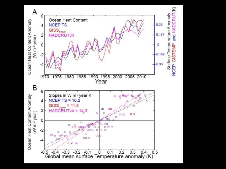
• Observations of the covariability of global mean surface temperature and ASR/OLR give statistically significant estimates of λSW and λLW • λSW = 0. 8 ± 0. 4 W m-2 K-1 • λLW = -2. 0 ± 0. 3 W m-2 K-1

Implications for OLR recovery timescale • Observational constraints suggest that τcross is of order decades IN RESPONSE TO LW FORCING ONLY • Assumes an (CMIP 5 ensemble average) radiative relaxation timescale (τ) of 27 years τCROSS = τ ln(-λ LW / λ SW )
?")
Can we get climate feedbacks from interannual variability of CERES (and surface temperature)?

Radiation causes surface temperature anomalies as well as responds to it– potential to confuse the nonfeedback forcing with the feedback.

Conclusions CO 2 initiates global warming by decreasing OLR but the TOA energy imbalance is dominated by increased absorbed solar radiation in most climate models – associated with surface albedo and SW water vapor feedbacks CERES data also suggest a positive shortwave feedback global warming will most likely result in enhanced ASR and we should not expect to see reduced OLR from the forcing Can interannual variability in CERES tell us anything about climate feedbacks?

How to reconcile this – response to greenhouse forcing with a shortwave feedback LW feedback only Greenhouse forcing FLW= 4 W m-2 ΔOLR =0 -λLW ΔT = 4 W m-2 ΔT= 2 K Forcing = response FLW = -λLW ΔT if λLW = -2 W m -2 K -1 ΔT = FLW /-λLW = 2 K LW and SW feedback FLW= 4 W m-2 λSW ΔT = 4 W m-2 ΔT= 4 K λLW ΔT = 8 W m-2 ΔOLR= -FLW + -λLW ΔT = ΔASR Forcing = response FLW = -(λLW +λSW ) ΔT if λSW = +1 W m -2 K -1 ΔT = FLW /-(λLW + λSW ) = 4 K

Time evolution of OLR response to greenhouse forcing with SW feedback OLR must go from –FLW at time 0 to FLW in the equilibrium response ASR OLR returns to unperturbed value OLR FLW The energy imbalance equation: Has the solution: when half of the equilibrium temperature change occurs

Are the radiative feedbacks that operate on inter-annual timescales equivalent to equilibrium feedbacks? SW LW NET
")
Water Vapor as a SW Absorber (Figure: Robert Rhode Global Warming Art Project)

Heat capacity: 4 XCO 2 • Heat capacity increases with time as energy penetrates into the ocean • In first couple decades, energy is within the first couple 100 m of ocean and system e-folds to radiative equilibrium in about a decade

How fast does the system approach equilibrium? Ensemble average forcing and feedbacks • C = 250 m (30 W m-2 year K-1) the ensemble average for first century after forcing • λLW = -1. 7 W m-2 K-1 • λSW = +0. 6 W m-2 K-1 The energy imbalance equation: Has the solution: Key point: OLR returns to unperturbed value in of order the radiative relaxation timescale of the system decades

What parameter controls inter. GCM spread in TOA response? • Using all GCM specific parameters gets the inter-model spread in τcross • Varying just λSW and FSW between GCMS captures inter-model spread in τcross • λLW , FLW and heat capacity differences between GCMs less important for determining the radiative response • Varying just λSW gives bi-modal distribution of τcross with exception of two models (FSW plays a role here)

τcross dependence on feedback parameters Ensemble average forcing and feedbacks • λLW = -1. 7 W m-2 K-1 • λSW = +0. 6 W m-2 K-1 • FLW = + 6. 1 W m-2 equilibrium temperature change initial final transition OLR =0 at τ=τcross How far from equilibrium OLR =0
: Ensemble Average τcross")
Sensitivity of τCROSS to feedback parameters If FSW = 0 (simplification): Ensemble Average τcross is determined by the OLR value demanded in the new equilibrium Set by relative magnitudes of λ LW and λ SW HAS STEEP GRADIENTS IN

What parameter controls inter. GCM spread in TOA response? • While the relative magnitudes of λSW and λLW explain the vast majority of the spread in τcross there are several model outliers • A more complete analysis includes inter-model differences in FSW (small) clouds FSW includes both direct radiative forcing by CO 2 and the rapid response of to the forcing

From before, if FSW =0 then: : Feedback Gain = 2 If |λSW| = ½ |λLW| TEQ is doubled The OLR change to get to equilibrium is: (2*FLW/ |λLW|) * |λLW| = 2 FLW OLR = 0 occurs half way to equilibrium TCROSS = T ln(2) If FSW ≠ 0 then: : Forcing Gain = 2 If FLW = FSW TEQ is doubled and OLR asymptotes to +FLW OLR = 0 occurs half way to equilibrium TCROSS = T ln(2)

SW and LW Feedbacks and Forcing: 4 XCO 2 Feedbacks LW SW Ensembl e Average Forcing • LW feedback is negative (stabilizing) and has small inter. GCM spread • SW feedback is mostly positive and has large inter-GCM spread • Forcing is mostly in LW (greenhouse) • SW forcing has a significant inter -GCM spread

Sensitivity of τCROSS to feedback parameters • Positive SW forcing and feedbacks favor a short OLR recovery timescale with a symetric dependence on the “gain” factors • Explains the majority (R= 0. 88) of inter- model spread • Assumes a time and model invariant heat capacity (250 m ocean depth equivalent)

• LW Feedback parameter from observations Surface temperature explains a small fraction of OLR’ variance (R=0. 52) • Error bars on regression coefficient (1σ) are small, why? • Weak 1 month auto-correlation in OLR’ – r. OLR (1 month) = 0. 3 lots of DOF (N*= 113) Unexplained amplitude Independent realizations Even if none of the OLR’ variance was explained, the regression slope is still significant Given the number of realizations, you would seldom realize such a large regression coefficient in a random sample – in the absence of a genuine relationship between TS and OLR
 • Almost")
• SW Feedback parameter from observations Very weak correlation (r=0. 16) • Almost no memory in ASR’ – r. OLR (1 month) = 0. 1 – mean we have lots of DOF (N*= 143) The significance of the regression slope is not a consequence of the variance explained but, rather, the non-zero of the slope despite the number of realizations The feedback has emerged from the non-feedback radiative processes in the record
- Slides: 39