Shortest Paths Algorithms for standard variants Algorithms and

Shortest Paths: Algorithms for standard variants Algorithms and Networks 2017/2018 Johan M. M. van Rooij Hans L. Bodlaender 1

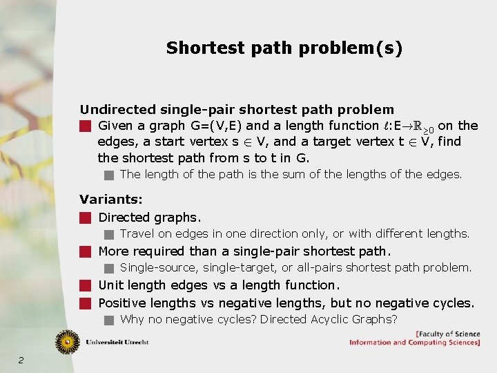
Shortest path problem(s) Undirected single-pair shortest path problem g Given a graph G=(V, E) and a length function l: E!R¸ 0 on the edges, a start vertex s 2 V, and a target vertex t 2 V, find the shortest path from s to t in G. g The length of the path is the sum of the lengths of the edges. Variants: g Directed graphs. g Travel on edges in one direction only, or with different lengths. g More required than a single-pair shortest path. g Single-source, single-target, or all-pairs shortest path problem. g Unit length edges vs a length function. g Positive lengths vs negative lengths, but no negative cycles. g Why no negative cycles? Directed Acyclic Graphs? 2

Shortest paths and other courses g Algorithms course (Bachelor, level 3) g Dijkstra. g Bellman-Ford. g Floyd-Warshall. g Crowd simulation course (Master, period 2) g Previously known as the course ‘Path Planning’. g A* and bidirectional Dijkstra (maybe also other courses). g Many extensions to this. 3

Shortest paths in algorithms and networks g This lecture: g Recap on what you should know. • Floyd-Warshall. • Bellman-Ford. • Dijkstra. g Using height functions. • Optimisation to Dijkstra: A* and bidirectional search. • Johnson’s algorithm (all-pairs). g Next week: g Gabow’s algorithm (using the numbers). g Large scale shortest paths algorithms in practice. • Contraction hierarchies. • Partitioning using natural cuts. 4

Applications g Route planning. g Shortest route from A to B. g Subproblem in vehicle routing problems. g Preprocessing for travelling salesman problem on graphs. g Subroutine in other graph algorithms. g Preprocessing in facility location problems. g Subproblem in several flow algorithms. g Many other problems can be modelled a shortest path problems. g State based problems where paths are sequences of state transitions. g Longest paths on directed acyclic graphs. 5

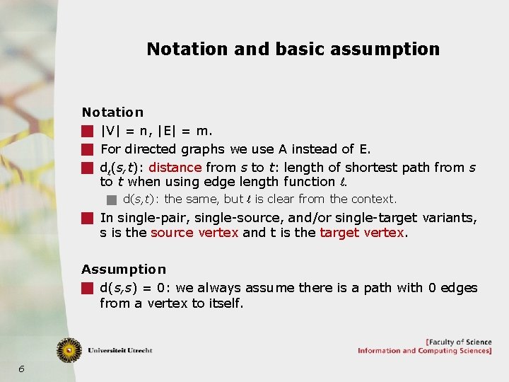
Notation and basic assumption Notation g |V| = n, |E| = m. g For directed graphs we use A instead of E. g dl(s, t): distance from s to t: length of shortest path from s to t when using edge length function l. g d(s, t): the same, but l is clear from the context. g In single-pair, single-source, and/or single-target variants, s is the source vertex and t is the target vertex. Assumption g d(s, s) = 0: we always assume there is a path with 0 edges from a vertex to itself. 6

Shortest Paths – Algorithms and Networks RECAP ON ALGORITHMS YOU SHOULD KNOW 7

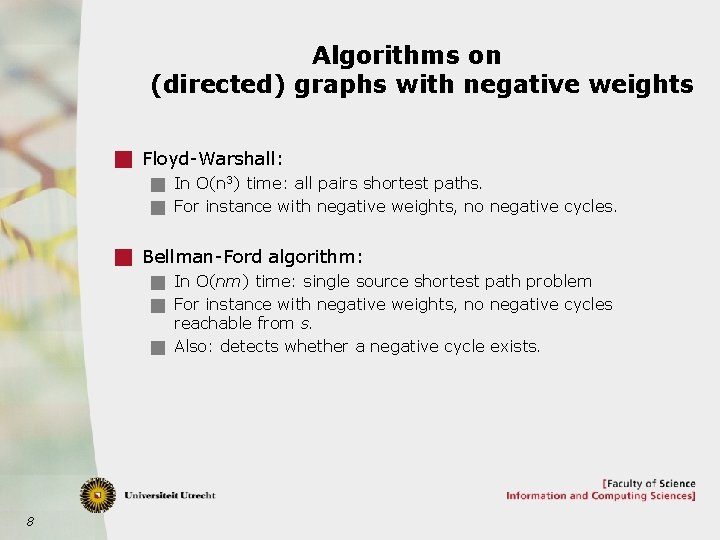
Algorithms on (directed) graphs with negative weights g Floyd-Warshall: g In O(n 3) time: all pairs shortest paths. g For instance with negative weights, no negative cycles. g Bellman-Ford algorithm: g In O(nm) time: single source shortest path problem g For instance with negative weights, no negative cycles reachable from s. g Also: detects whether a negative cycle exists. 8

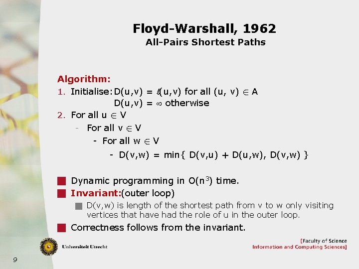
Floyd-Warshall, 1962 All-Pairs Shortest Paths Algorithm: 1. Initialise: D(u, v) = l(u, v) for all (u, v) 2 A D(u, v) = ¥ otherwise 2. For all u 2 V - For all v 2 V - For all w 2 V - D(v, w) = min{ D(v, u) + D(u, w), D(v, w) } g Dynamic programming in O(n 3) time. g Invariant: (outer loop) g D(v, w) is length of the shortest path from v to w only visiting vertices that have had the role of u in the outer loop. g Correctness follows from the invariant. 9

Bellman-Ford algorithm, 1956 Single source for graphs with negative lengths 1. Initialize: set D[v] = ¥ for all v 2 V{s}. set D[s] = 0 (s is the source). 2. Repeat |V|-1 times: Clearly: O(nm) time g For every edge (u, v) 2 A: D[v] = min{ D[v], D[u]+ l(u, v) }. 3. For every edge (u, v) 2 A g If D[v] > D[u] + l(u, v) then there exists a negative cycle. g Invariant: If there is no negative cycle reachable from s, then after i runs of main loop, we have: g If there is a shortest path from s to u with at most i edges, then D[u]=d(s, u), for all u. g If there is no negative cycle reachable from s, then every vertex has a shortest path with at most n – 1 edges. g If there is a negative cycle reachable from s, then there will always be an edge where an update step is possible. 10

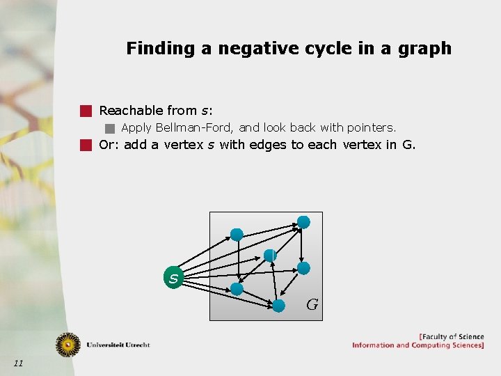
Finding a negative cycle in a graph g Reachable from s: g Apply Bellman-Ford, and look back with pointers. g Or: add a vertex s with edges to each vertex in G. s G 11

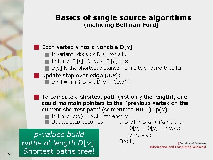
Basics of single source algorithms (including Bellman-Ford) g Each vertex v has a variable D[v]. g Invariant: d(s, v) £ D[v] for all v g Initially: D[s]=0; v¹ s: D[v] = ¥. g D[v] is the shortest distance from s to v found thus far. g Update step over edge (u, v): g D[v] = min{ D[v], D[u]+ l(u, v) }. g To compute a shortest path (not only the length), one could maintain pointers to the `previous vertex on the current shortest path’ (sometimes NULL): p(v). g Initially: p(v) = NULL for each v. g Update step becomes: If D[v] > D[u]+ l(u, v) then 12 p-values build paths of length D[v]. Shortest paths tree! D[v] = D[u] + l(u, v); p(v) = u; End if;

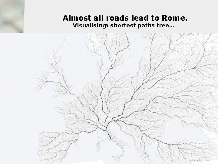
Almost all roads lead to Rome. Visualisinga shortest paths tree… g Theorem: Almost all roads lead to Rome. g Proof: g … 13

What Rome? 14

Dijkstra’s algorithm, 1956 Dijkstra’s Algorithm 1. Initialize: set D[v] = ¥ for all v 2 V{s}, D[s] = 0. 2. Take priority queue Q, initially containing all vertices. 3. While Q is not empty, g Select vertex v from Q with minimum value D[v]. g Update D[u] across all outgoing edges (v, u). • D[v] = min{ D[v], D[u]+ l(u, v) }. g Update the priority queue Q for all such u. g Assumes all lengths are non-negative. g Correctness proof (done in `Algoritmiek’ course). g Note: if all edges have unit-length, then this becomes Breath-First Search. g Priority queue only has priorities 1 and ¥. 15

On Dijkstra’s algorithm g Running time depends on the data structure chosen for the priority queue. g Selection happens at most n times. g Updates happen at most m times. Depending on the data structure used, the running time is: g O(n 2): array. g Selection in O(n) time, updates in O(1) time. g O((m + n) log n): Red-black tree (or other), heap. g Selection and updates in O(log n). g O(m + n log n): Fibonacci heaps. g Selection (delete min) in amortised O(log n), update in amortised O(1) time. 16

Shortest Paths – Algorithms and Networks OPTIMISATIONS FOR DIJKSTRA’S ALGORITHM 17

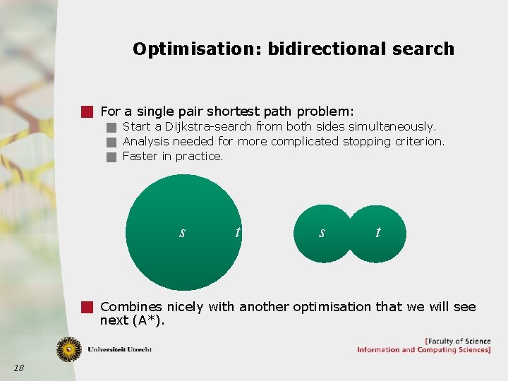
Optimisation: bidirectional search g For a single pair shortest path problem: g Start a Dijkstra-search from both sides simultaneously. g Analysis needed for more complicated stopping criterion. g Faster in practice. s t g Combines nicely with another optimisation that we will see next (A*). 18

A* g Consider shortest paths in geometric setting. g For example: route planning for car system. g Standard Dijkstra would explore many paths that are clearly in the wrong direction. g Utrecht to Groningen would look at roads near Den Bosch or even Maastricht. g A* modifies the edge length function used to direct Dijkstra’s algorithm into the right direction. g To do so, we will use a heuristic as a height function. 19

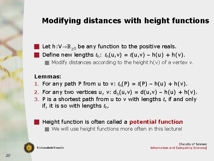
Modifying distances with height functions g Let h: V!R¸ 0 be any function to the positive reals. g Define new lengths lh: lh(u, v) = l(u, v) – h(u) + h(v). g Modify distances according to the height h(v) of a vertex v. Lemmas: 1. For any path P from u to v: lh(P) = l(P) – h(u) + h(v). 2. For any two vertices u, v: dh(u, v) = d(u, v) – h(u) + h(v). 3. P is a shortest path from u to v with lengths l, if and only if, it is so with lengths lh. g Height function is often called a potential function. g We will use height functions more often in this lecture! 20

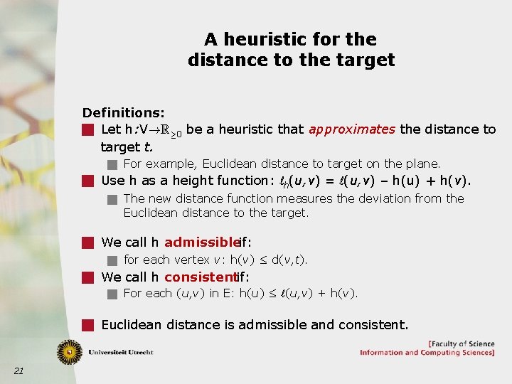
A heuristic for the distance to the target Definitions: g Let h: V!R¸ 0 be a heuristic that approximates the distance to target t. g For example, Euclidean distance to target on the plane. g Use h as a height function: lh(u, v) = l(u, v) – h(u) + h(v). g The new distance function measures the deviation from the Euclidean distance to the target. g We call h admissibleif: g for each vertex v: h(v) ≤ d(v, t). g We call h consistentif: g For each (u, v) in E: h(u) ≤ l(u, v) + h(v). g Euclidean distance is admissible and consistent. 21

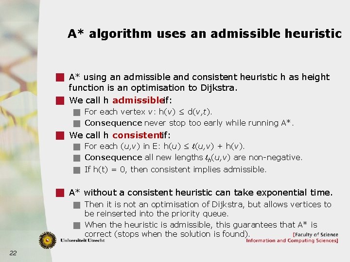
A* algorithm uses an admissible heuristic g A* using an admissible and consistent heuristic h as height function is an optimisation to Dijkstra. g We call h admissibleif: g For each vertex v: h(v) ≤ d(v, t). g Consequence : never stop too early while running A*. g We call h consistentif: g For each (u, v) in E: h(u) ≤ l(u, v) + h(v). g Consequence : all new lengths lh(u, v) are non-negative. g If h(t) = 0, then consistent implies admissible. g A* without a consistent heuristic can take exponential time. g Then it is not an optimisation of Dijkstra, but allows vertices to be reinserted into the priority queue. g When the heuristic is admissible, this guarantees that A* is correct (stops when the solution is found). 22

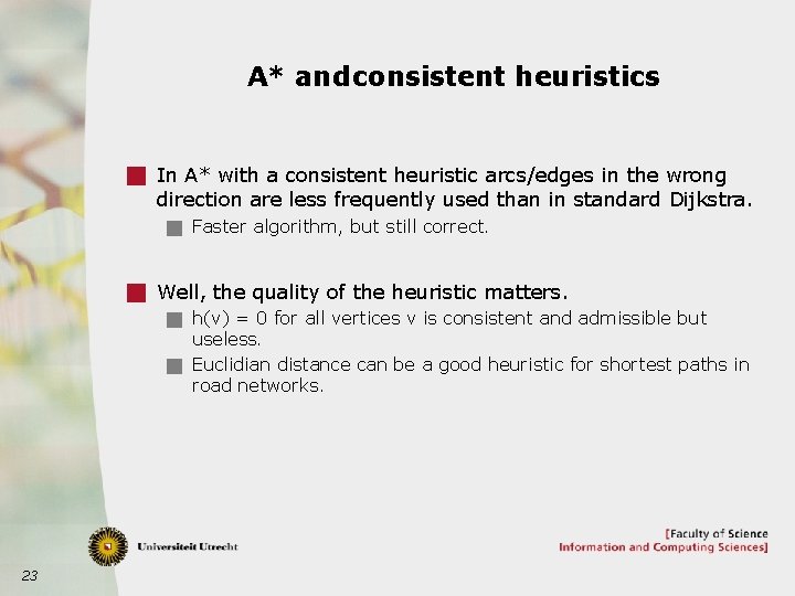
A* and consistent heuristics g In A* with a consistent heuristic arcs/edges in the wrong direction are less frequently used than in standard Dijkstra. g Faster algorithm, but still correct. g Well, the quality of the heuristic matters. g h(v) = 0 for all vertices v is consistent and admissible but useless. g Euclidian distance can be a good heuristic for shortest paths in road networks. 23

Advanced Shortest Path Algorithms and Networks 2017/2018 Johan M. M. van Rooij Hans L. Bodlaender 24

New Planning for Shortest Paths Subjects g Last week: g Recap on what you should know. • Floyd-Warshall. • Bellman-Ford. • Dijkstra. g Using height functions. • Optimisation to Dijkstra: A* and bidirectional search. g This lecture : g Johnson’s algorithm (all-pairs). g Gabow’s algorithm (using the numbers). g Probably in the T. B. A. slot in week 50 (before first exam). g Large scale shortest paths algorithms in practice. • Contraction hierarchies • Partitioning using natural cuts. 25

Shortest Paths - Algorithms and Networks JOHNSON’S ALGORITHM 26

All Pairs Shortest Paths: Johnson’s Algorithm Observation g If all weights are non-negative we can run Dijkstra with each vertex as starting vertex. g This gives O(n 2 log n + nm) time using a Fibonacci heap. g On sparse graphs, this is faster than the O(n 3) of Floyd- Warshall. g Johnson: all-pairs shortest paths improvement for sparse graphs with reweighting technique: g O(n 2 log n + nm) time. g Works with negative lengths, but no negative cycles. g Reweighting using height functions. 27

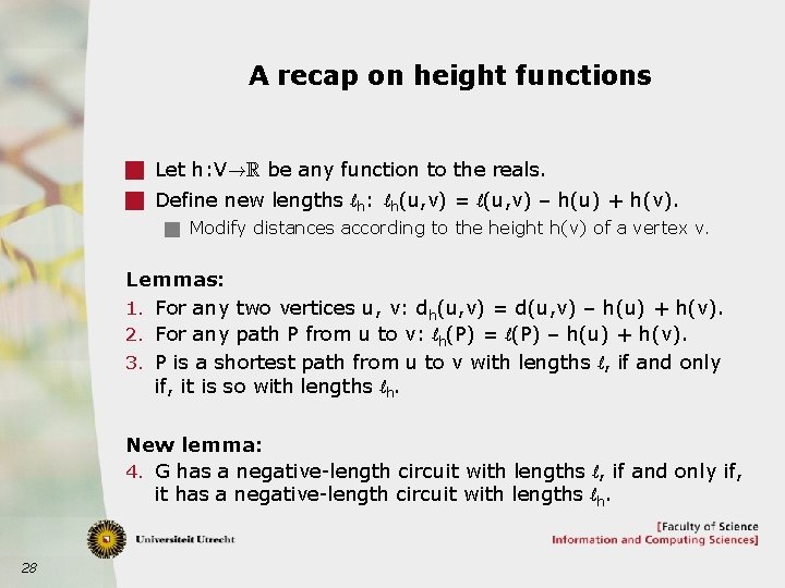
A recap on height functions g Let h: V!R be any function to the reals. g Define new lengths lh: lh(u, v) = l(u, v) – h(u) + h(v). g Modify distances according to the height h(v) of a vertex v. Lemmas: 1. For any two vertices u, v: dh(u, v) = d(u, v) – h(u) + h(v). 2. For any path P from u to v: lh(P) = l(P) – h(u) + h(v). 3. P is a shortest path from u to v with lengths l, if and only if, it is so with lengths lh. New lemma: 4. G has a negative-length circuit with lengths l, if and only if, it has a negative-length circuit with lengths lh. 28

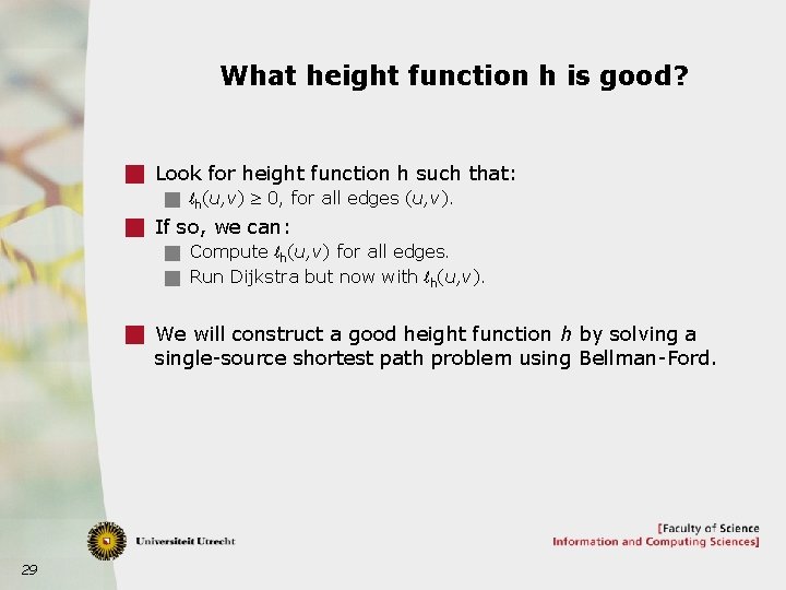
What height function h is good? g Look for height function h such that: g lh(u, v) ³ 0, for all edges (u, v). g If so, we can: g Compute lh(u, v) for all edges. g Run Dijkstra but now with lh(u, v). g We will construct a good height function h by solving a single-source shortest path problem using Bellman-Ford. 29

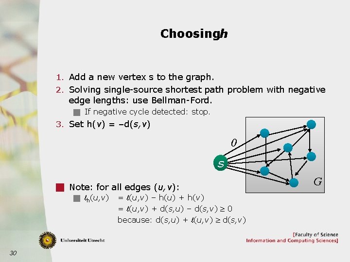
Choosingh 1. Add a new vertex s to the graph. 2. Solving single-source shortest path problem with negative edge lengths: use Bellman-Ford. g If negative cycle detected: stop. 3. Set h(v) = –d(s, v) 0 s g Note: for all edges (u, v): g lh(u, v) = l(u, v) – h(u) + h(v) = l(u, v) + d(s, u) – d(s, v) ³ 0 because: d(s, u) + l(u, v) ³ d(s, v) 30 G

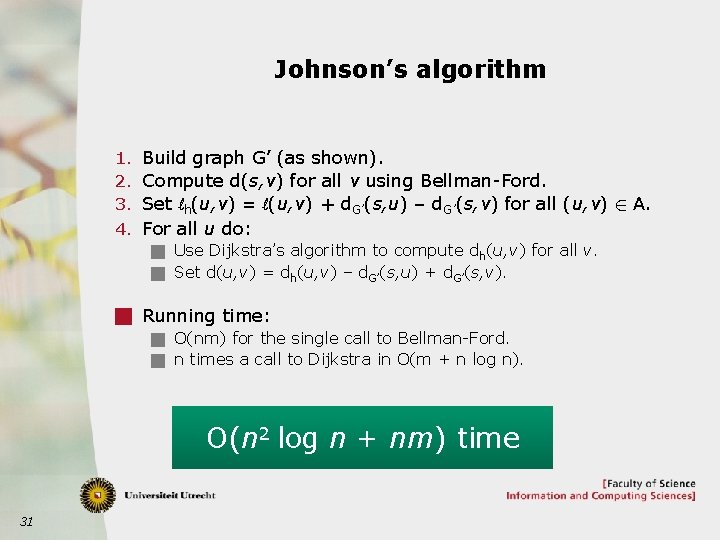
Johnson’s algorithm 1. Build graph G’ (as shown). 2. Compute d(s, v) for all v using Bellman-Ford. 3. Set lh(u, v) = l(u, v) + d. G’(s, u) – d. G’(s, v) for all (u, v) 2 A. 4. For all u do: g Use Dijkstra’s algorithm to compute dh(u, v) for all v. g Set d(u, v) = dh(u, v) – d. G’(s, u) + d. G’(s, v). g Running time: g O(nm) for the single call to Bellman-Ford. g n times a call to Dijkstra in O(m + n log n). O(n 2 log n + nm) time 31

Shortest Paths - Algorithms and Networks GABOW’S ALGORITHM: USING THE NUMBERS 32

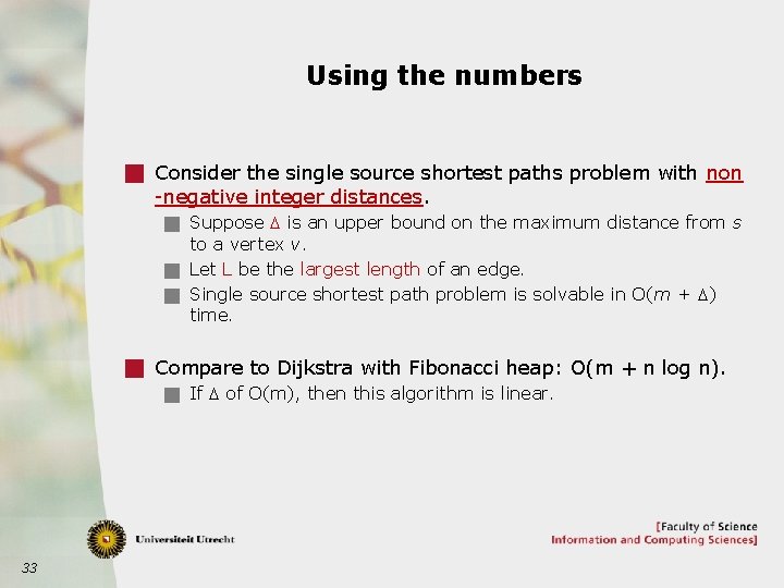
Using the numbers g Consider the single source shortest paths problem with non -negative integer distances. g Suppose D is an upper bound on the maximum distance from s to a vertex v. g Let L be the largest length of an edge. g Single source shortest path problem is solvable in O(m + D) time. g Compare to Dijkstra with Fibonacci heap: O(m + n log n). g If D of O(m), then this algorithm is linear. 33

In O(m+D) time g We use Dijkstra, using D[v] for length of the shortest path found thus far, using the following as a priority queue. 1. Keep array of doubly linked lists: L[0], …, L[D]. g Invariant: for all v with D[v] £ D: v is in L[D[v]]. 2. Keep a current minimum m. g Invariant : all L[k] with k < m are empty. g Run ‘Dijkstra’ while: g Update D[v] from x to y: take v from L[x], and add it to L[y]. This takes O(1) time each. g Extract min: while L[m] empty, m ++; then take the first element from list L[m]. g Total time: O(m+D) 34

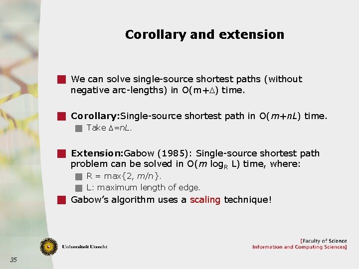
Corollary and extension g We can solve single-source shortest paths (without negative arc-lengths) in O(m+D) time. g Corollary: Single-source shortest path in O(m+n. L) time. g Take D=n. L. g Extension: Gabow (1985): Single-source shortest path problem can be solved in O(m log. R L) time, where: g R = max{2, m/n}. g L: maximum length of edge. g Gabow’s algorithm uses a scaling technique! 35

Gabow’s Algorithm: Main Idea Sketch of the algorithm: g First, build a scaled instance: g For each edge e set l’(e) = ë l(e) / R û. g Recursively, solve the scaled instance and switch to using Dijkstra ‘using the numbers’ if weights are small enough. g R * dl’(s, v) is when we scale back our scaled instance. g We want d(s, v). g What error did we make while rounding? g Another shortest paths instance can be used to compute the error correction terms on the shortest paths! g How does this work? See next slides. 36

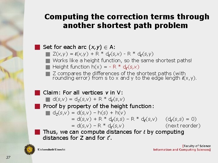
Computing the correction terms through another shortest path problem g Set for each arc (x, y) 2 A: g Z(x, y) = l(x, y) + R * dl’(s, x) - R * dl’(s, y) g Works like a height function, so the same shortest paths! g Height function h(x) = - R * dl’(s, x) g Z compares the differences of the shortest paths (with rounding error) from s to x and y to the edge length l(x, y). g Claim: For all vertices v in V: g d(s, v) = d. Z(s, v) + R * dl’(s, v) g Proof by property of the height function: g d. Z(s, v) = d(s, v) – h(s) + h(v) = d(s, v) + R * dl’(s, s) – R * dl’(s, v) (dl’(s, s) = 0) = d(s, v) – R * dl’(s, v) (next reorder) g Thus, we can compute distances for l by computing distances for Z and for l’. 37

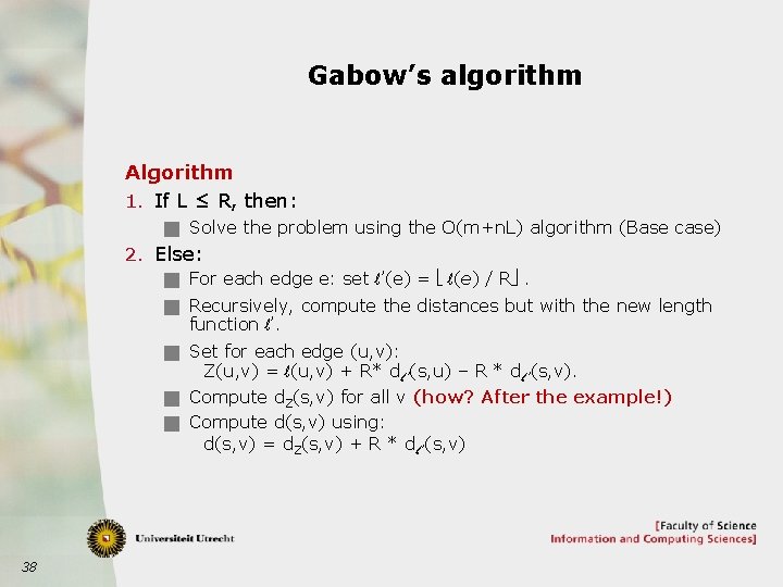
Gabow’s algorithm Algorithm 1. If L ≤ R, then: g Solve the problem using the O(m+n. L) algorithm (Base case) 2. Else: g For each edge e: set l’(e) = ë l(e) / Rû. g Recursively, compute the distances but with the new length function l’. g Set for each edge (u, v): Z(u, v) = l(u, v) + R* dl ’(s, u) – R * dl ’(s, v). g Compute d. Z(s, v) for all v (how? After the example!) g Compute d(s, v) using: d(s, v) = d. Z(s, v) + R * dl ’(s, v) 38

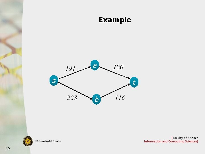
Example 191 a 180 s t 223 39 b 116

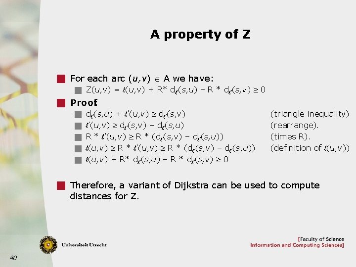
A property of Z g For each arc (u, v) Î A we have: g Z(u, v) = l(u, v) + R* dl’(s, u) – R * dl’(s, v) ³ 0 g Proof: g dl’(s, u) + l’(u, v) ³ dl’(s, v) g l’(u, v) ³ dl’(s, v) – dl’(s, u) g R * l’(u, v) ³ R * (dl’(s, v) – dl’(s, u)) g l(u, v) ³ R * l’(u, v) ³ R * (dl’(s, v) – dl’(s, u)) g l(u, v) + R* dl’(s, u) – R * dl’(s, v) ³ 0 (triangle inequality) (rearrange). (times R). (definition of l(u, v)) g Therefore, a variant of Dijkstra can be used to compute distances for Z. 40

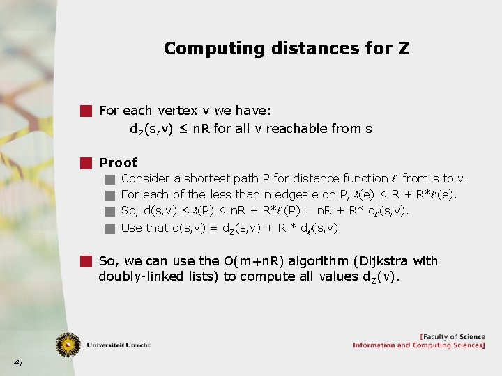
Computing distances for Z g For each vertex v we have: d. Z(s, v) ≤ n. R for all v reachable from s g Proof: g Consider a shortest path P for distance function l’ from s to v. g For each of the less than n edges e on P, l(e) ≤ R + R*l’(e). g So, d(s, v) ≤ l(P) ≤ n. R + R*l’(P) = n. R + R* dl’(s, v). g Use that d(s, v) = d. Z(s, v) + R * dl’(s, v). g So, we can use the O(m+n. R) algorithm (Dijkstra with doubly-linked lists) to compute all values d. Z(v). 41

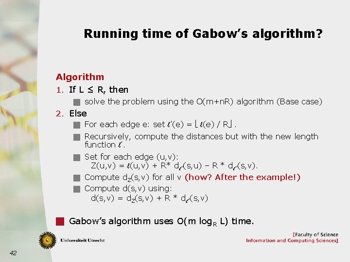
Running time of Gabow’s algorithm? Algorithm 1. If L ≤ R, then g solve the problem using the O(m+n. R) algorithm (Base case) 2. Else g For each edge e: set l’(e) = ë l(e) / Rû. g Recursively, compute the distances but with the new length function l’. g Set for each edge (u, v): Z(u, v) = l(u, v) + R* dl ’(s, u) – R * dl ’(s, v). g Compute d. Z(s, v) for all v (how? After the example!) g Compute d(s, v) using: d(s, v) = d. Z(s, v) + R * dl ’(s, v) g Gabow’s algorithm uses O(m log. R L) time. 42

Large Scale Practical Shortest Path Algorithms and Networks 2017/2018 Johan M. M. van Rooij Hans L. Bodlaender 44

Large scale shortest paths algorithms g The world’s road network is huge. g Open street map has: 2, 750, 000 nodes. g Standard (bidirectional) Dijkstra takes too long. g Many-to-many computations are very challenging. g We briefly consider two algorithms. g Contraction Hierarchies. g Partitioning through natural cuts. g Both algorithms have two phases. g Time consuming preprocessing phase. g Very fast shortest paths queries. g My goal: give you a rough idea on these algorithms. g Look up further details if you want to. 45

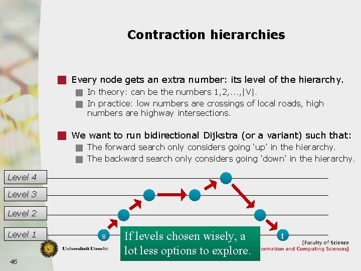
Contraction hierarchies g Every node gets an extra number: its level of the hierarchy. g In theory: can be the numbers 1, 2, . . . , |V|. g In practice: low numbers are crossings of local roads, high numbers are highway intersections. g We want to run bidirectional Dijkstra (or a variant) such that: g The forward search only considers going ‘up’ in the hierarchy. g The backward search only considers going ‘down’ in the hierarchy. Level 4 Level 3 Level 2 Level 1 46 s If levels chosen wisely, a lot less options to explore. t

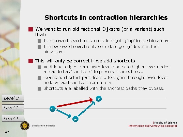
Shortcuts in contraction hierarchies g We want to run bidirectional Dijkstra (or a variant) such that: g The forward search only considers going ‘up’ in the hierarchy. g The backward search only considers going ‘down’ in the hierarchy. g This will only be correct if we add shortcuts. g Additional edges from lower level nodes to higher level nodes are added as ‘shortcuts’ to preserve correctness. g Example: shortest path from u to v goes through lower level node w: add shortcut from u to v. g Shortcuts are labelled with the shortest paths they bypass. Level 3 Level 2 Level 1 47 v u w

Preprocessing for contraction hierarchies Preprocessing phase: g Assign a level to each node. g For each node, starting from the lowest level nodes upwards: g Consider it’s adjacent nodes of higher level and check whether the shortest path between these two nodes goes through the current node. g If so, add a shortcut edge between the adjacent nodes. g Great way of using preprocessing to accelerate lots of shortest paths computations. g But: g This preprocessing is very expensive on huge graphs. g Resulting graph can have many more edges (space requirement). g If the graph changes locally, lots of recomputation required. 48

Partitioning using natural cuts Observation g Shortest paths from cities in Brabant to cities above the rivers have little options of crossing the rivers. g This is a natural small-cut in the graph. g Many such cuts exist at various levels: g Sea’s, rivers, canals, . . . g Mountains, hills, . . . g Country-borders, village borders, . . . g Etc. . . 49

Example of natural cuts From: Delling, Goldberg, Razenshteyn, Werneck. Graph Partitioning with Natural Cuts. 50

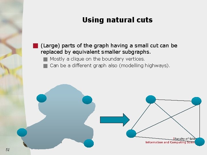
Using natural cuts g (Large) parts of the graph having a small cut can be replaced by equivalent smaller subgraphs. g Mostly a clique on the boundary vertices. g Can be a different graph also (modelling highways). 51

Computing shortest paths using natural cuts g When computing shortest paths: g For s and t, compute the distance to all partition-boundary vertices of the corresponding partition. g Replace all other partitions by their simplifications. g Graph is much smaller than the original graph. g This idea can be used hierarchically. g First partition at the continent/country level. g Partition each part into smaller parts. g Etc. g Finding good partitions with small natural cuts at the lowest level is easy. g Finding a good hierarchy is difficult. 52

Finding natural cuts Repeat the following process a lot of times: g Pick a random vertex v. g Use breadth first search to find a group of vertices around v. g Stop when we have x vertices in total ! this is the core. g Continue until we have y vertices in total ! this is the ring. g Use max-flow min-cut to compute the min cut between the core and vertices outside the ring. g The resulting cut could be part of natural cut. g After enough repetitions: g We find lots of cuts, creating a lot of islands. g Recombine these islands to proper size partitions. g Recombining the islands to a useful hierarchy is difficult. 53

Conclusion on using natural cuts g Natural cuts preprocessing has the advantage that: g Space requirement less extreme than contraction hierarchies, because hierarchical partitioning of the graph into regions. g Local changes to the graph can be processed with less recomputation time. g Precomputation can also be used if travel times are departure time dependent. g Preprocessing is still very expensive on huge graphs. g Last year experimentation project : find a good algorithm for building a hierarchical natural cuts partioning on real data. g Conclusion: hierarchical partitioning is best using 2 -cuts. g Possible new experimentation/thesis project: g Find effective 2 -partitioning algorithms for this purpose. 54

Shortest Paths – Algorithms and Networks CONCLUSION 55

Summary on Shortest Paths g We have seen: g Recap on what you should know. • Floyd-Warshall. • Bellman-Ford. • Dijkstra. g Using height functions. • Optimisation to Dijkstra: A* and bidirectional search. • Johnson’s algorithm (all-pairs). g Gabow’s algorithm (using the numbers). g Large scale shortest paths algorithms in practice. • Contraction hierarchies. • Partitioning using natural cuts. g Any questions? 56