Shortcourse Compressive Sensing of Videos Venue CVPR 2012

![Spatio-angular tradeoff [Ng, 2005] Spatio-angular tradeoff [Ng, 2005]](https://slidetodoc.com/presentation_image_h/de6f757cee6fac9906e0a01ab94e1637/image-18.jpg)
![Spatio-angular tradeoff [Levoy et al. 2006] Spatio-angular tradeoff [Levoy et al. 2006]](https://slidetodoc.com/presentation_image_h/de6f757cee6fac9906e0a01ab94e1637/image-19.jpg)
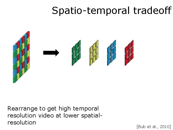
![Spatio-temporal tradeoff Stagger pixel-shutter within each exposure [Bub et al. , 2010] Spatio-temporal tradeoff Stagger pixel-shutter within each exposure [Bub et al. , 2010]](https://slidetodoc.com/presentation_image_h/de6f757cee6fac9906e0a01ab94e1637/image-20.jpg)
![Insight from the 70’s • Draw [Kashin, Gluskin] at random – iid Gaussian – Insight from the 70’s • Draw [Kashin, Gluskin] at random – iid Gaussian –](https://slidetodoc.com/presentation_image_h/de6f757cee6fac9906e0a01ab94e1637/image-46.jpg)
![Specialized solvers • Co. SAMP • SPG_l 1 [Needell and Tropp, 2009] [Friedlander, van Specialized solvers • Co. SAMP • SPG_l 1 [Needell and Tropp, 2009] [Friedlander, van](https://slidetodoc.com/presentation_image_h/de6f757cee6fac9906e0a01ab94e1637/image-65.jpg)

- Slides: 96

Short-course Compressive Sensing of Videos Venue CVPR 2012, Providence, RI, USA June 16, 2012 Organizers: Richard G. Baraniuk Mohit Gupta Aswin C. Sankaranarayanan Ashok Veeraraghavan

Part 2: Compressive sensing Motivation, theory, recovery • Linear inverse problems • Sensing visual signals • Compressive sensing – Theory – Hallmark – Recovery algorithms • Model-based compressive sensing – Models specific to visual signals

Linear inverse problems

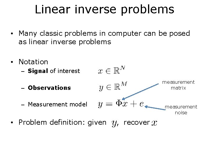
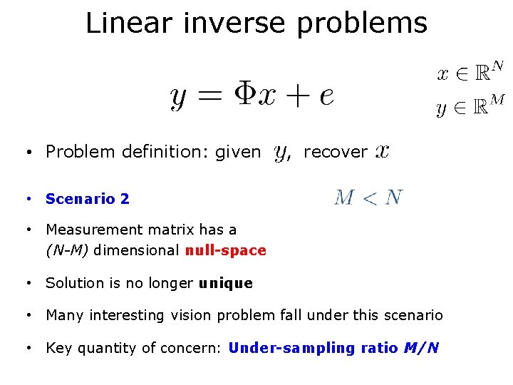
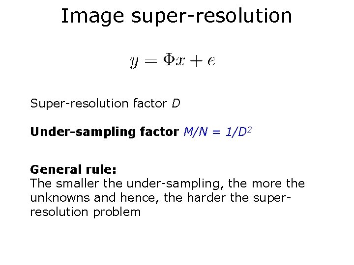
Linear inverse problems • Many classic problems in computer can be posed as linear inverse problems • Notation – Signal of interest measurement matrix – Observations – Measurement model • Problem definition: given measurement noise , recover

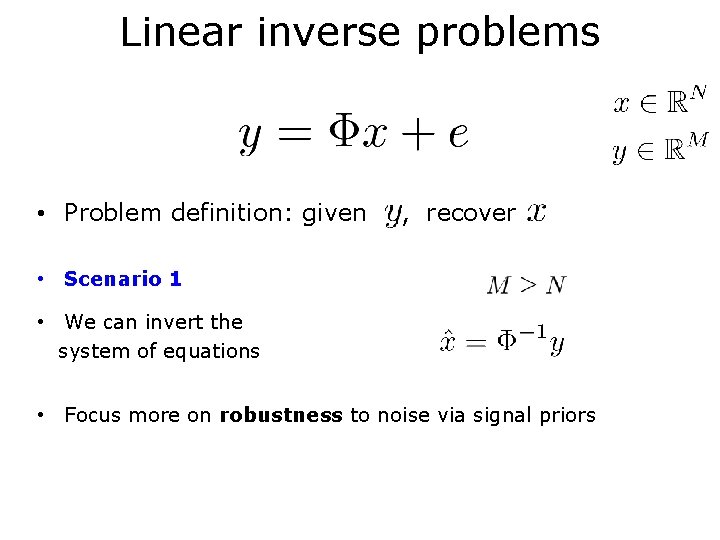
Linear inverse problems • Problem definition: given , recover • Scenario 1 • We can invert the system of equations • Focus more on robustness to noise via signal priors

Linear inverse problems • Problem definition: given , recover • Scenario 2 • Measurement matrix has a (N-M) dimensional null-space • Solution is no longer unique • Many interesting vision problem fall under this scenario • Key quantity of concern: Under-sampling ratio M/N

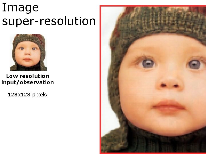
Image super-resolution Low resolution input/observation 128 x 128 pixels

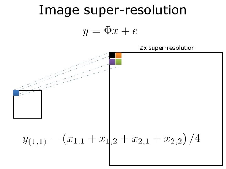
Image super-resolution 2 x super-resolution

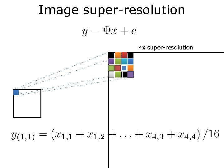
Image super-resolution 4 x super-resolution

Image super-resolution Super-resolution factor D Under-sampling factor M/N = 1/D 2 General rule: The smaller the under-sampling, the more the unknowns and hence, the harder the superresolution problem

Many other vision problems… • Affine rank minimizaiton, Matrix completion, deconvolution, Robust PCA • Image synthesis – Infilling, denoising, etc. • Light transport – Reflectance fields, BRDFs, Direct global separation, Light transport matrices • Sensing

Sensing visual signals

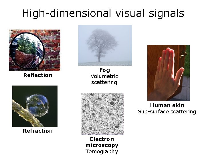
High-dimensional visual signals Reflection Fog Volumetric scattering Human skin Sub-surface scattering Refraction Electron microscopy Tomography

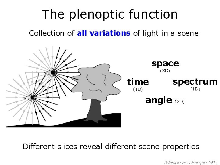
The plenoptic function Collection of all variations of light in a scene space (3 D) spectrum time (1 D) angle (2 D) Different slices reveal different scene properties Adelson and Bergen (91)

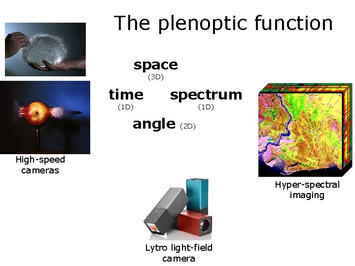
The plenoptic function space (3 D) time (1 D) spectrum (1 D) angle (2 D) High-speed cameras Hyper-spectral imaging Lytro light-field camera

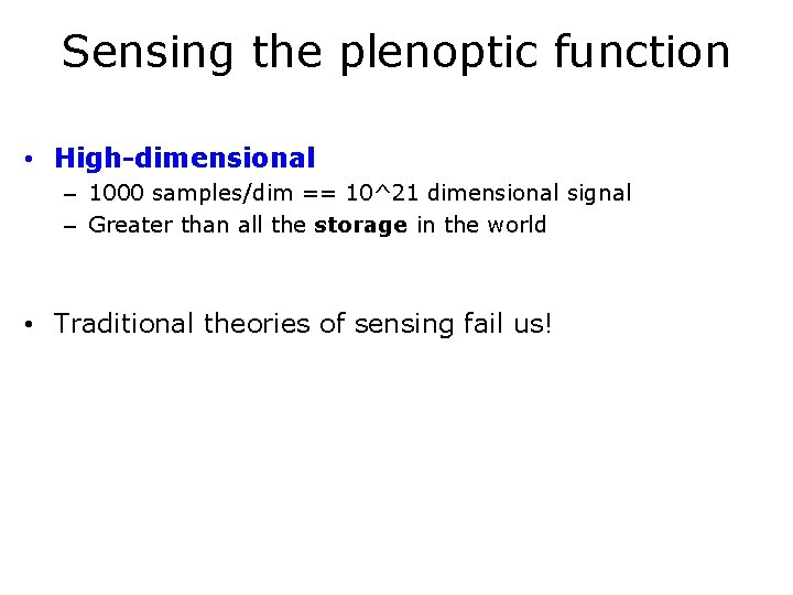
Sensing the plenoptic function • High-dimensional – 1000 samples/dim == 10^21 dimensional signal – Greater than all the storage in the world • Traditional theories of sensing fail us!

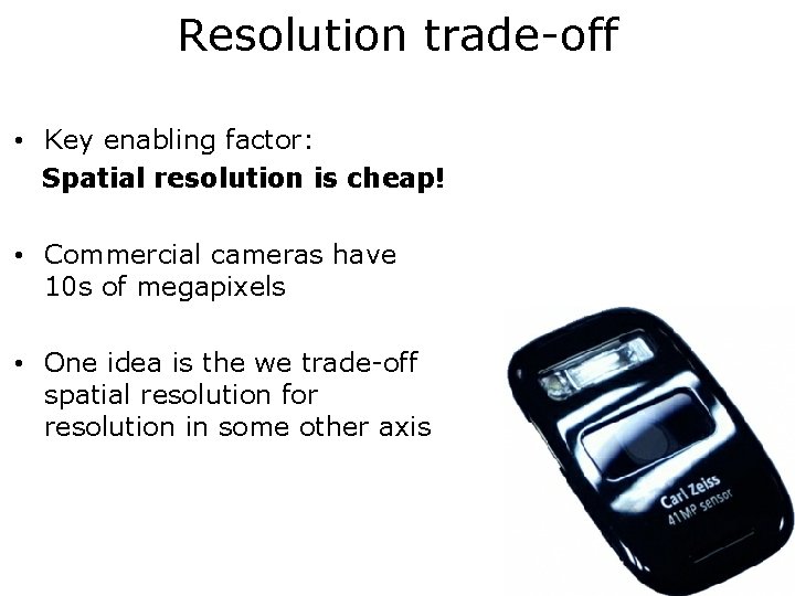
Resolution trade-off • Key enabling factor: Spatial resolution is cheap! • Commercial cameras have 10 s of megapixels • One idea is the we trade-off spatial resolution for resolution in some other axis
![Spatioangular tradeoff Ng 2005 Spatio-angular tradeoff [Ng, 2005]](https://slidetodoc.com/presentation_image_h/de6f757cee6fac9906e0a01ab94e1637/image-18.jpg)
Spatio-angular tradeoff [Ng, 2005]
![Spatioangular tradeoff Levoy et al 2006 Spatio-angular tradeoff [Levoy et al. 2006]](https://slidetodoc.com/presentation_image_h/de6f757cee6fac9906e0a01ab94e1637/image-19.jpg)
Spatio-angular tradeoff [Levoy et al. 2006]
![Spatiotemporal tradeoff Stagger pixelshutter within each exposure Bub et al 2010 Spatio-temporal tradeoff Stagger pixel-shutter within each exposure [Bub et al. , 2010]](https://slidetodoc.com/presentation_image_h/de6f757cee6fac9906e0a01ab94e1637/image-20.jpg)
Spatio-temporal tradeoff Stagger pixel-shutter within each exposure [Bub et al. , 2010]

Spatio-temporal tradeoff Rearrange to get high temporal resolution video at lower spatialresolution [Bub et al. , 2010]

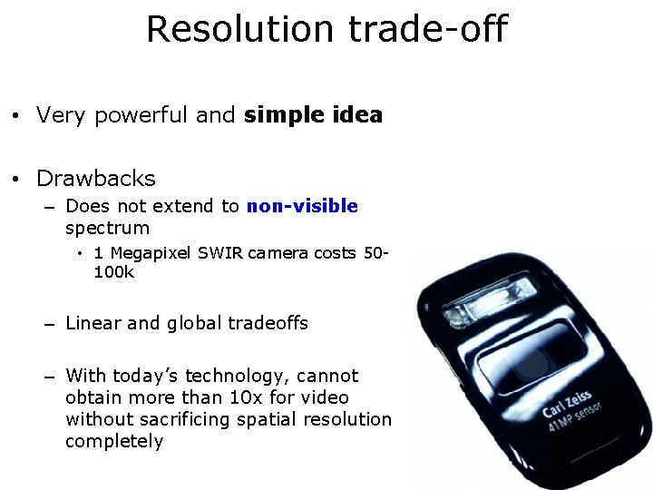
Resolution trade-off • Very powerful and simple idea • Drawbacks – Does not extend to non-visible spectrum • 1 Megapixel SWIR camera costs 50100 k – Linear and global tradeoffs – With today’s technology, cannot obtain more than 10 x for video without sacrificing spatial resolution completely

Compressive sensing

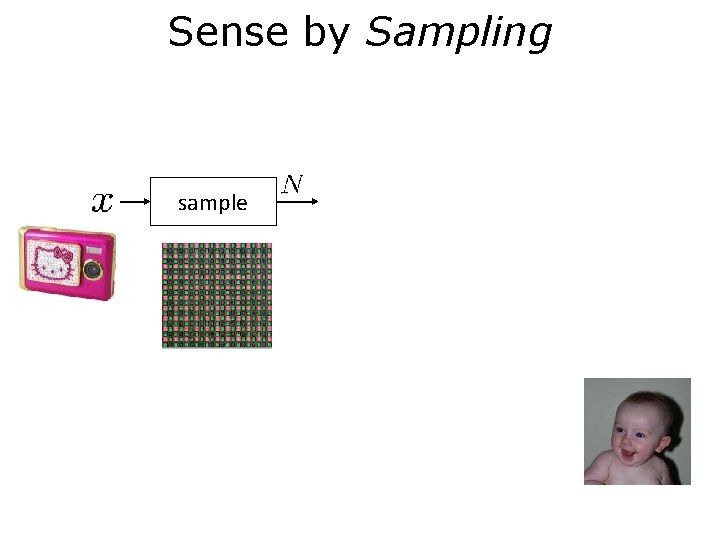
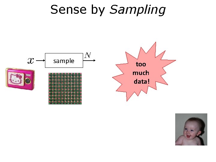
Sense by Sampling sample

Sense by Sampling sample too much data!

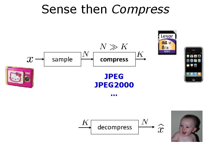
Sense then Compress sample compress JPEG 2000 … decompress

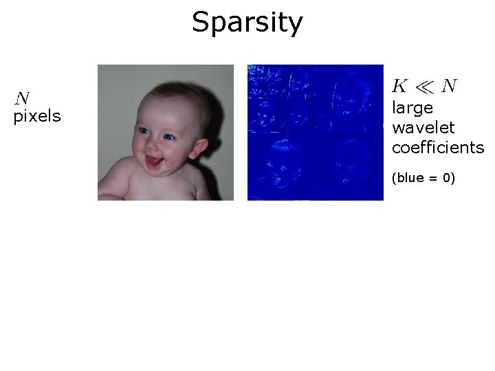
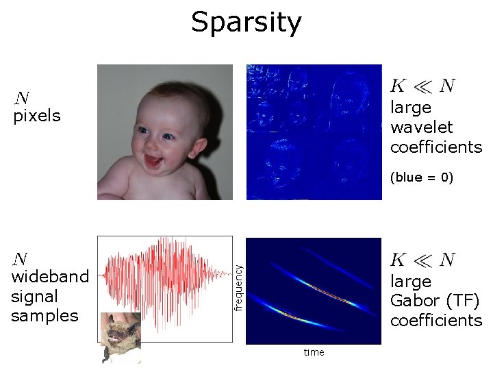
Sparsity pixels large wavelet coefficients (blue = 0)

Sparsity large wavelet coefficients pixels wideband signal samples frequency (blue = 0) large Gabor (TF) coefficients time

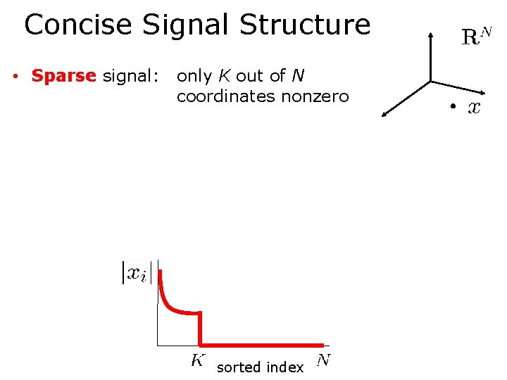
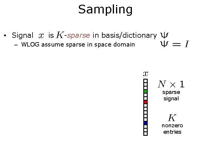
Concise Signal Structure • Sparse signal: only K out of N coordinates nonzero sorted index

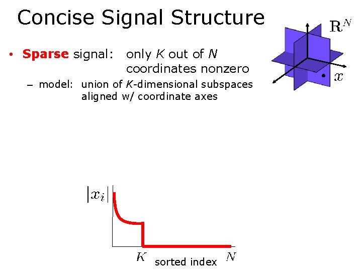
Concise Signal Structure • Sparse signal: only K out of N coordinates nonzero – model: union of K-dimensional subspaces aligned w/ coordinate axes sorted index

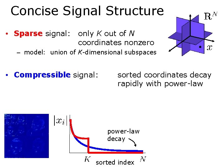
Concise Signal Structure • Sparse signal: only K out of N coordinates nonzero – model: union of K-dimensional subspaces • Compressible signal: sorted coordinates decay rapidly with power-law decay sorted index

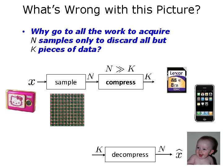
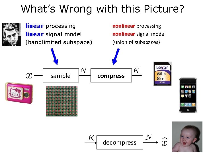
What’s Wrong with this Picture? • Why go to all the work to acquire N samples only to discard all but K pieces of data? sample compress decompress

What’s Wrong with this Picture? linear processing linear signal model (bandlimited subspace) sample nonlinear processing nonlinear signal model (union of subspaces) compress decompress

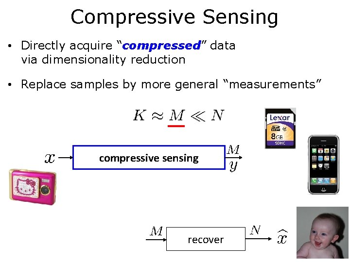
Compressive Sensing • Directly acquire “compressed” data via dimensionality reduction • Replace samples by more general “measurements” compressive sensing recover

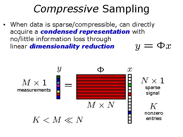
Sampling • Signal is -sparse in basis/dictionary – WLOG assume sparse in space domain sparse signal nonzero entries

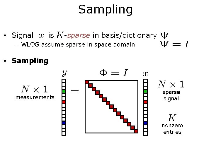
Sampling • Signal is -sparse in basis/dictionary – WLOG assume sparse in space domain • Sampling measurements sparse signal nonzero entries

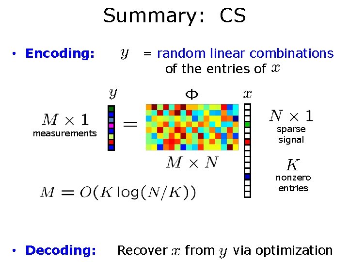
Compressive Sampling • When data is sparse/compressible, can directly acquire a condensed representation with no/little information loss through linear dimensionality reduction measurements sparse signal nonzero entries

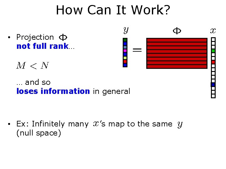
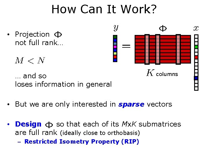
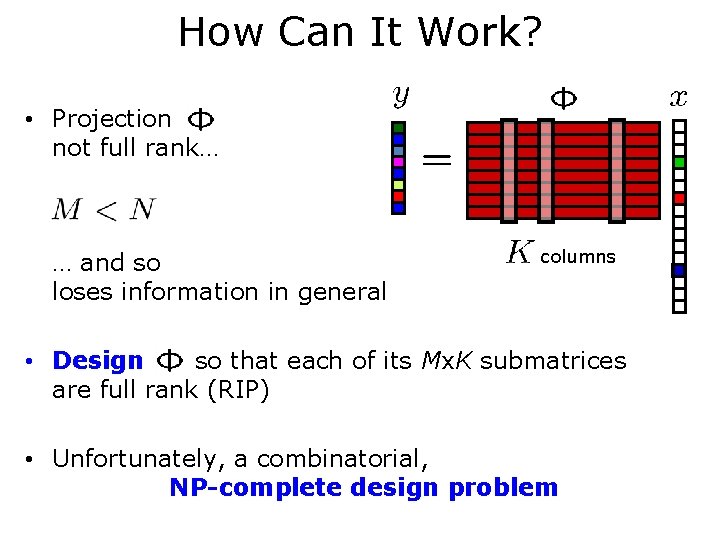
How Can It Work? • Projection not full rank… … and so loses information in general • Ex: Infinitely many (null space) ’s map to the same

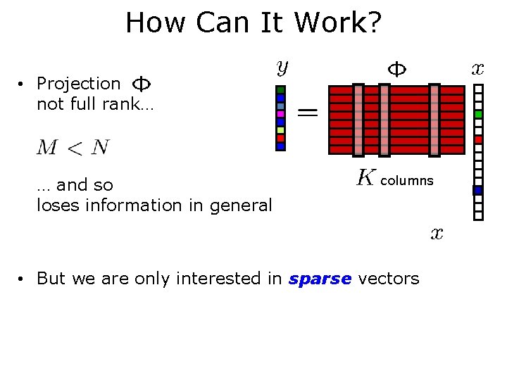
How Can It Work? • Projection not full rank… … and so loses information in general columns • But we are only interested in sparse vectors

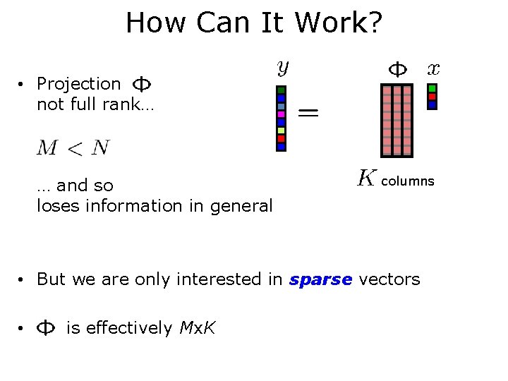
How Can It Work? • Projection not full rank… … and so loses information in general columns • But we are only interested in sparse vectors • is effectively Mx. K

How Can It Work? • Projection not full rank… … and so loses information in general columns • But we are only interested in sparse vectors • Design so that each of its Mx. K submatrices are full rank (ideally close to orthobasis) – Restricted Isometry Property (RIP)

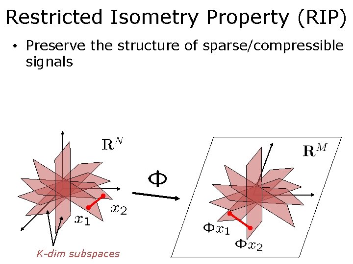
Restricted Isometry Property (RIP) • Preserve the structure of sparse/compressible signals K-dim subspaces

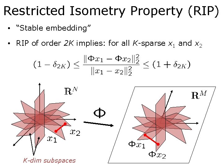
Restricted Isometry Property (RIP) • “Stable embedding” • RIP of order 2 K implies: for all K-sparse x 1 and x 2 K-dim subspaces

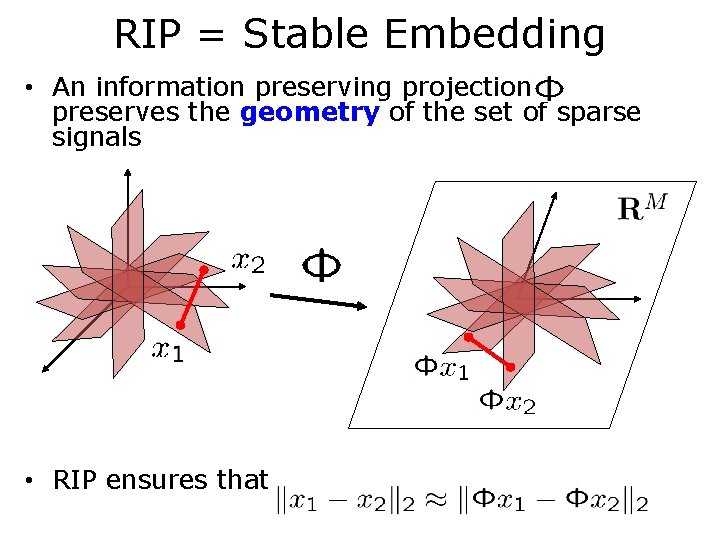
RIP = Stable Embedding • An information preserving projection preserves the geometry of the set of sparse signals • RIP ensures that

How Can It Work? • Projection not full rank… … and so loses information in general columns • Design so that each of its Mx. K submatrices are full rank (RIP) • Unfortunately, a combinatorial, NP-complete design problem
![Insight from the 70s Draw Kashin Gluskin at random iid Gaussian Insight from the 70’s • Draw [Kashin, Gluskin] at random – iid Gaussian –](https://slidetodoc.com/presentation_image_h/de6f757cee6fac9906e0a01ab94e1637/image-46.jpg)
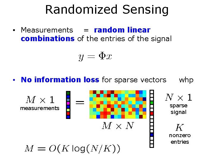
Insight from the 70’s • Draw [Kashin, Gluskin] at random – iid Gaussian – iid Bernoulli … columns • Then has the RIP with high probability provided

Randomized Sensing • Measurements = random linear combinations of the entries of the signal • No information loss for sparse vectors measurements whp sparse signal nonzero entries

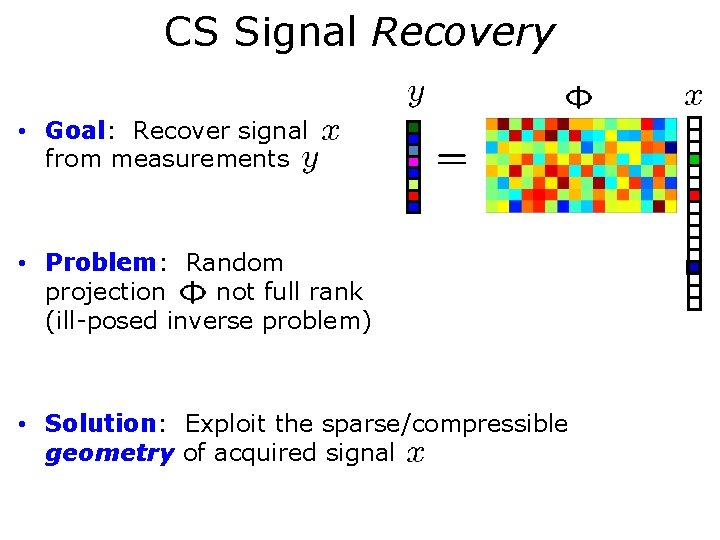
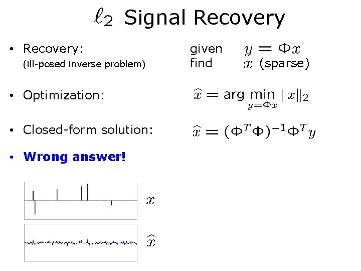
CS Signal Recovery • Goal: Recover signal from measurements • Problem: Random projection not full rank (ill-posed inverse problem) • Solution: Exploit the sparse/compressible geometry of acquired signal

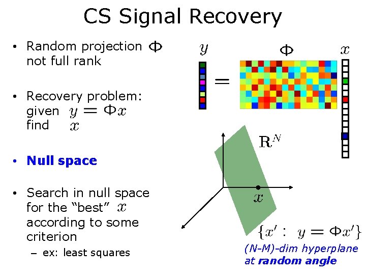
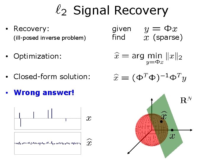
CS Signal Recovery • Random projection not full rank • Recovery problem: given find • Null space • Search in null space for the “best” according to some criterion – ex: least squares (N-M)-dim hyperplane at random angle

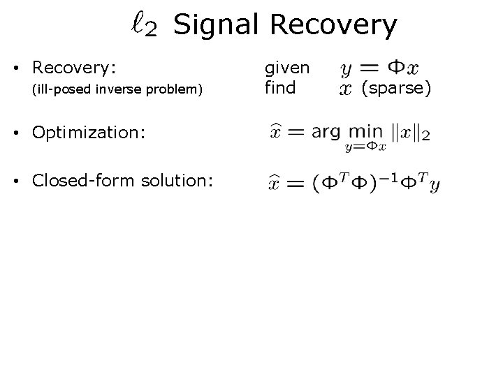
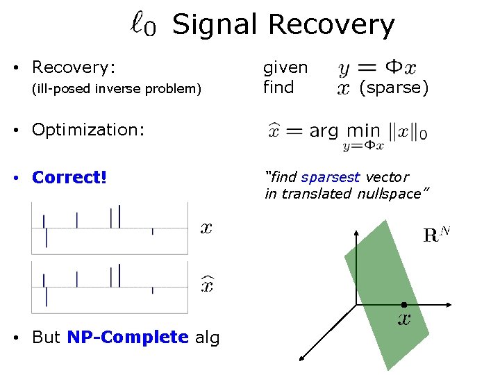
Signal Recovery • Recovery: (ill-posed inverse problem) • Optimization: • Closed-form solution: given find (sparse)

Signal Recovery • Recovery: (ill-posed inverse problem) • Optimization: • Closed-form solution: • Wrong answer! given find (sparse)

Signal Recovery • Recovery: (ill-posed inverse problem) • Optimization: • Closed-form solution: • Wrong answer! given find (sparse)

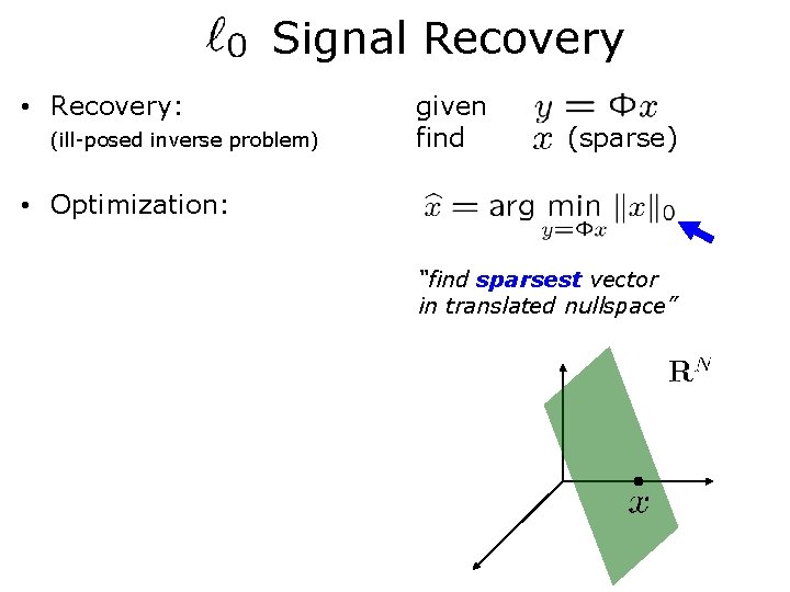
Signal Recovery • Recovery: (ill-posed inverse problem) given find (sparse) • Optimization: “find sparsest vector in translated nullspace”

Signal Recovery • Recovery: (ill-posed inverse problem) given find (sparse) • Optimization: • Correct! • But NP-Complete alg “find sparsest vector in translated nullspace”

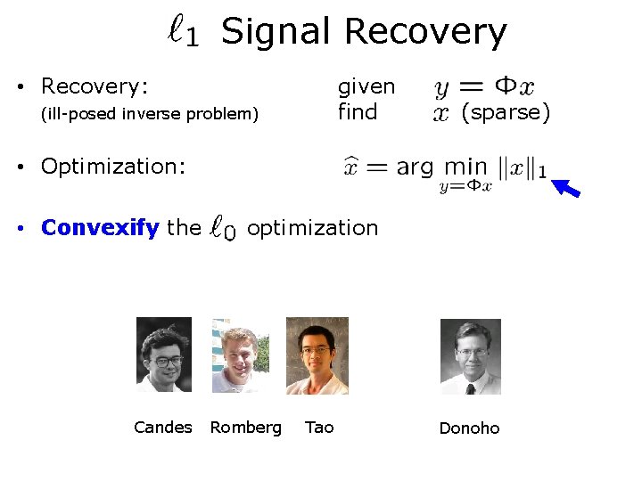
Signal Recovery • Recovery: given find (ill-posed inverse problem) (sparse) • Optimization: • Convexify the Candes optimization Romberg Tao Donoho

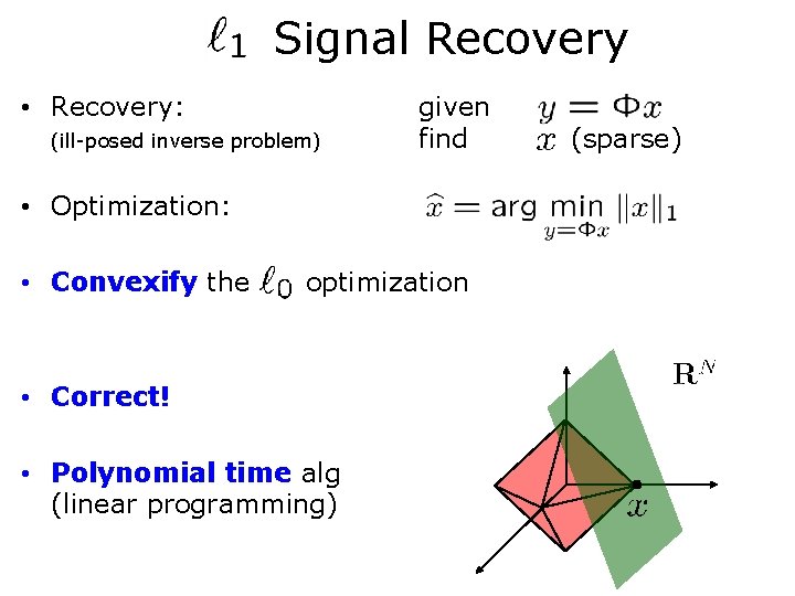
Signal Recovery • Recovery: (ill-posed inverse problem) given find • Optimization: • Convexify the optimization • Correct! • Polynomial time alg (linear programming) (sparse)

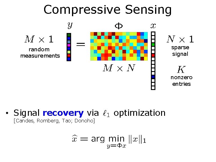
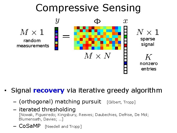
Compressive Sensing sparse signal random measurements nonzero entries • Signal recovery via [Candes, Romberg, Tao; Donoho] optimization

Compressive Sensing sparse signal random measurements nonzero entries • Signal recovery via iterative greedy algorithm – (orthogonal) matching pursuit – iterated thresholding [Gilbert, Tropp] [Nowak, Figueiredo; Kingsbury, Reeves; Daubechies, Defrise, De Mol; Blumensath, Davies; …] – Co. Sa. MP [Needell and Tropp]

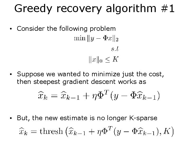
Greedy recovery algorithm #1 • Consider the following problem • Suppose we wanted to minimize just the cost, then steepest gradient descent works as • But, the new estimate is no longer K-sparse

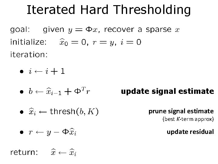
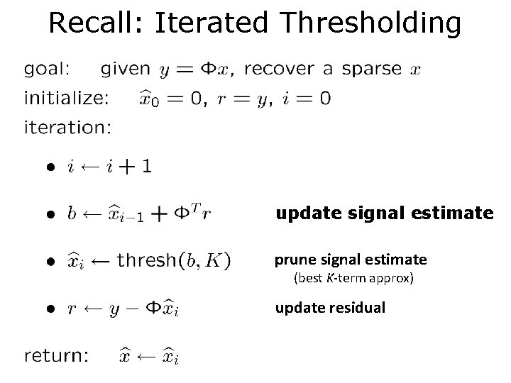
Iterated Hard Thresholding update signal estimate prune signal estimate (best K-term approx) update residual

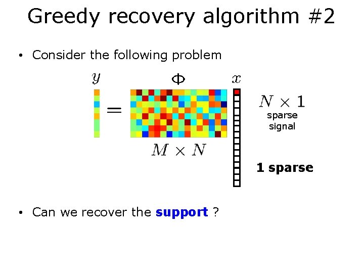
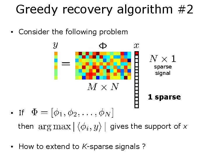
Greedy recovery algorithm #2 • Consider the following problem sparse signal 1 sparse • Can we recover the support ?

Greedy recovery algorithm #2 • Consider the following problem sparse signal 1 sparse • If then gives the support of x • How to extend to K-sparse signals ?

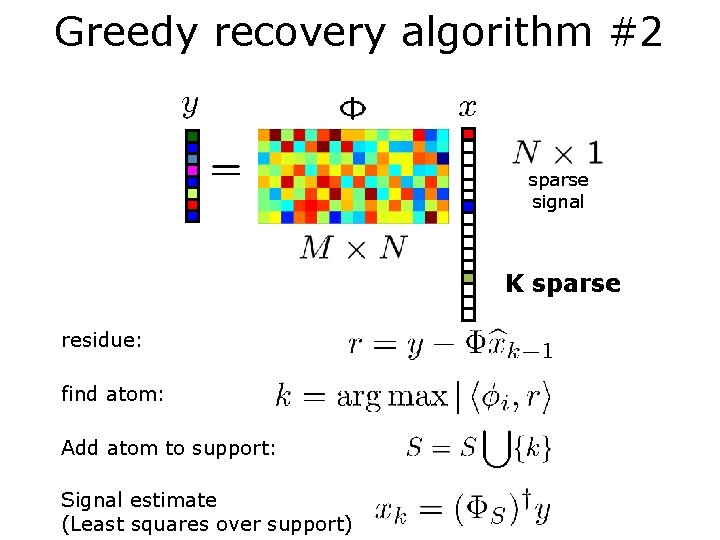
Greedy recovery algorithm #2 sparse signal K sparse residue: find atom: Add atom to support: Signal estimate (Least squares over support)

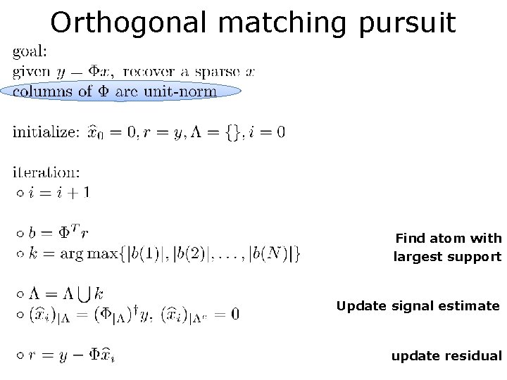
Orthogonal matching pursuit Find atom with largest support Update signal estimate update residual
![Specialized solvers Co SAMP SPGl 1 Needell and Tropp 2009 Friedlander van Specialized solvers • Co. SAMP • SPG_l 1 [Needell and Tropp, 2009] [Friedlander, van](https://slidetodoc.com/presentation_image_h/de6f757cee6fac9906e0a01ab94e1637/image-65.jpg)
Specialized solvers • Co. SAMP • SPG_l 1 [Needell and Tropp, 2009] [Friedlander, van der Berg, 2008] http: //www. cs. ubc. ca/labs/scl/spgl 1/ • FPC [Hale, Yin, and Zhang, 2007] http: //www. caam. rice. edu/~optimization/L 1/fpc/ • AMP [Donoho, Montanari and Maleki, 2010] many others, see dsp. rice. edu/cs and https: //sites. google. com/site/igorcarron 2/cscodes

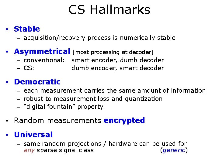
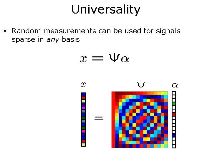
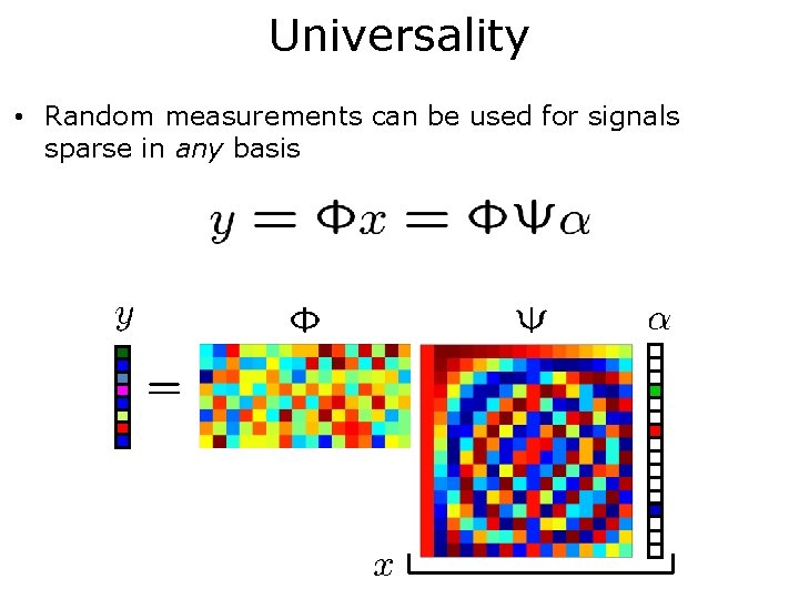
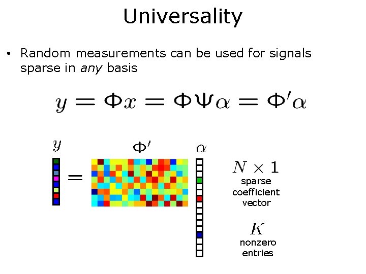
CS Hallmarks • Stable – acquisition/recovery process is numerically stable • Asymmetrical – conventional: – CS: (most processing at decoder) smart encoder, dumb decoder dumb encoder, smart decoder • Democratic – each measurement carries the same amount of information – robust to measurement loss and quantization – “digital fountain” property • Random measurements encrypted • Universal – same random projections / hardware can be used for any sparse signal class (generic)

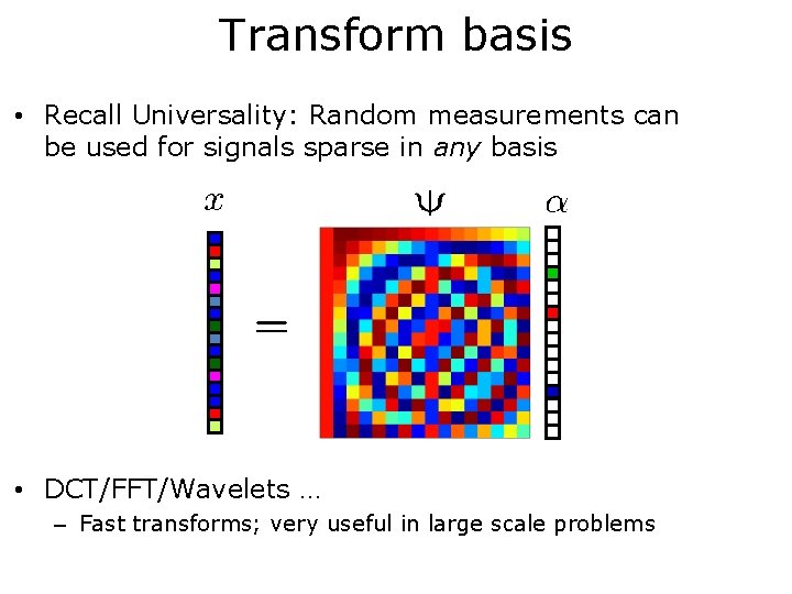
Universality • Random measurements can be used for signals sparse in any basis

Universality • Random measurements can be used for signals sparse in any basis

Universality • Random measurements can be used for signals sparse in any basis sparse coefficient vector nonzero entries

Summary: CS • Compressive sensing – randomized dimensionality reduction – exploits signal sparsity information – integrates sensing, compression, processing • Why it works: with high probability, random projections preserve information in signals with concise geometric structures – sparse signals – compressible signals

Summary: CS • Encoding: = random linear combinations of the entries of sparse signal measurements nonzero entries • Decoding: Recover from via optimization

Image/Video specific signal models and recovery algorithms

Transform basis • Recall Universality: Random measurements can be used for signals sparse in any basis • DCT/FFT/Wavelets … – Fast transforms; very useful in large scale problems

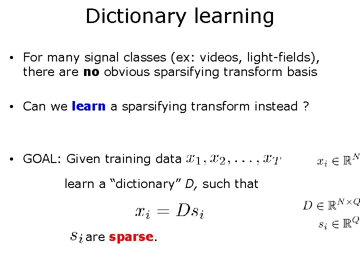
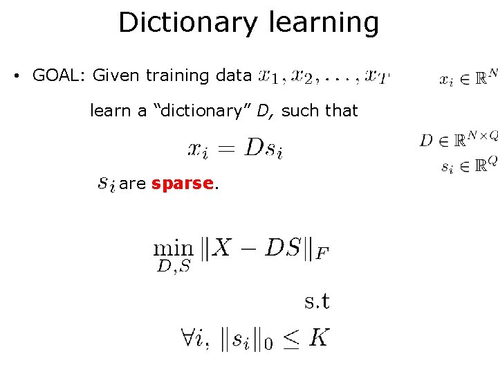
Dictionary learning • For many signal classes (ex: videos, light-fields), there are no obvious sparsifying transform basis • Can we learn a sparsifying transform instead ? • GOAL: Given training data learn a “dictionary” D, such that are sparse.

Dictionary learning • GOAL: Given training data learn a “dictionary” D, such that are sparse.

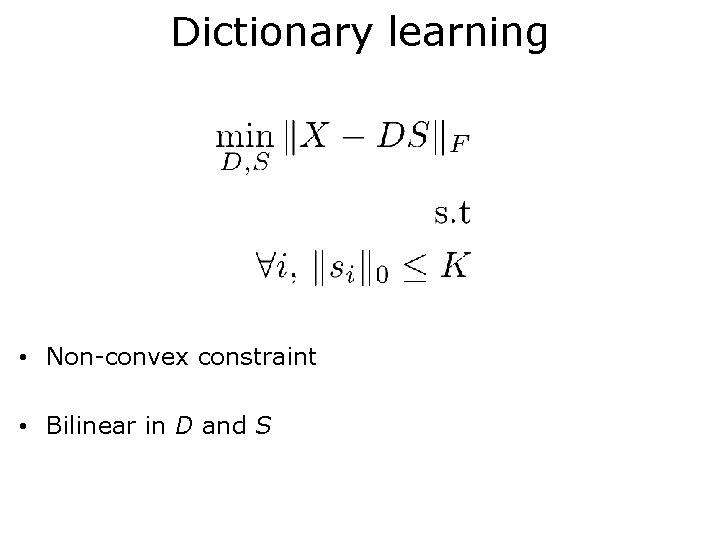
Dictionary learning • Non-convex constraint • Bilinear in D and S

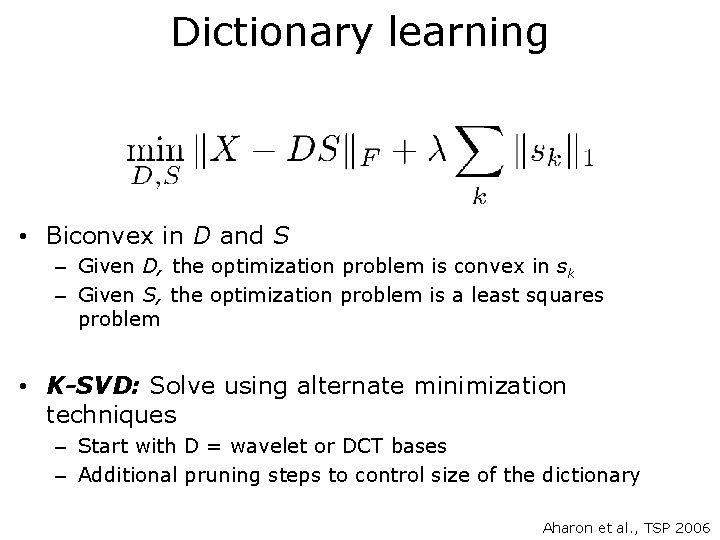
Dictionary learning • Biconvex in D and S – Given D, the optimization problem is convex in sk – Given S, the optimization problem is a least squares problem • K-SVD: Solve using alternate minimization techniques – Start with D = wavelet or DCT bases – Additional pruning steps to control size of the dictionary Aharon et al. , TSP 2006

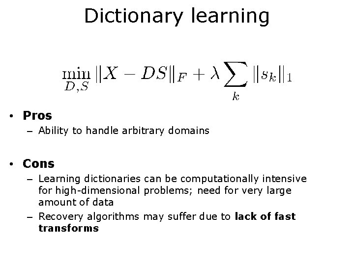
Dictionary learning • Pros – Ability to handle arbitrary domains • Cons – Learning dictionaries can be computationally intensive for high-dimensional problems; need for very large amount of data – Recovery algorithms may suffer due to lack of fast transforms

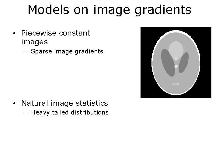
Models on image gradients • Piecewise constant images – Sparse image gradients • Natural image statistics – Heavy tailed distributions

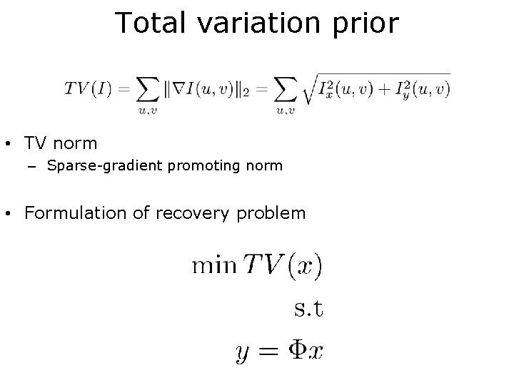
Total variation prior • TV norm – Sparse-gradient promoting norm • Formulation of recovery problem

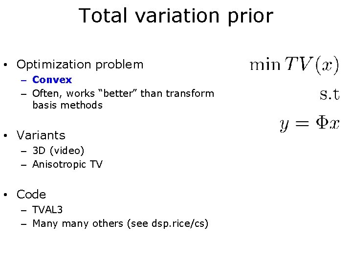
Total variation prior • Optimization problem – Convex – Often, works “better” than transform basis methods • Variants – 3 D (video) – Anisotropic TV • Code – TVAL 3 – Many many others (see dsp. rice/cs)

Beyond sparsity Model-based CS

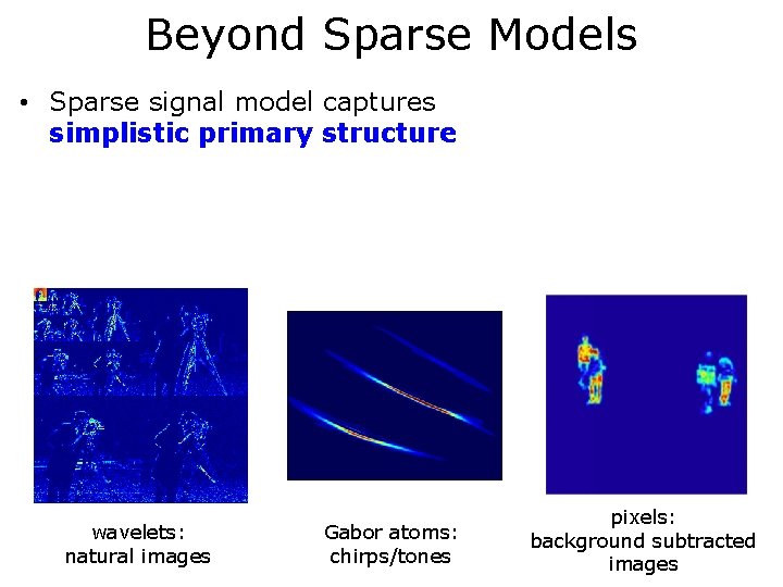
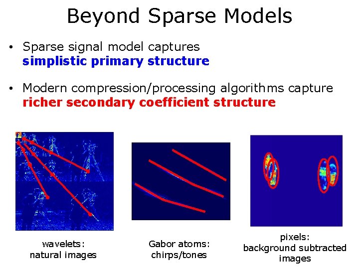
Beyond Sparse Models • Sparse signal model captures simplistic primary structure wavelets: natural images Gabor atoms: chirps/tones pixels: background subtracted images

Beyond Sparse Models • Sparse signal model captures simplistic primary structure • Modern compression/processing algorithms capture richer secondary coefficient structure wavelets: natural images Gabor atoms: chirps/tones pixels: background subtracted images

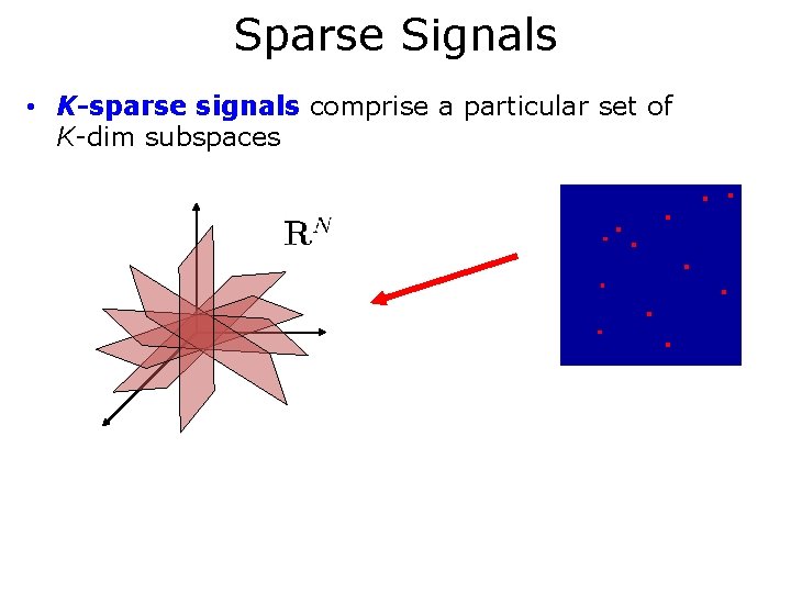
Sparse Signals • K-sparse signals comprise a particular set of K-dim subspaces

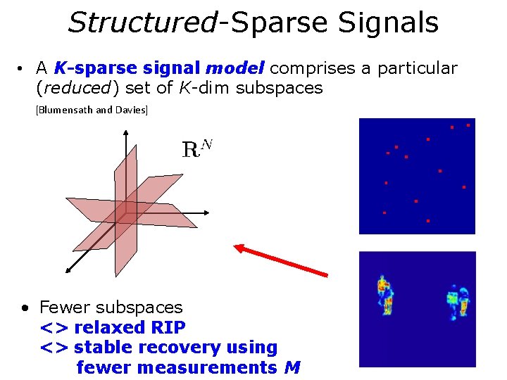
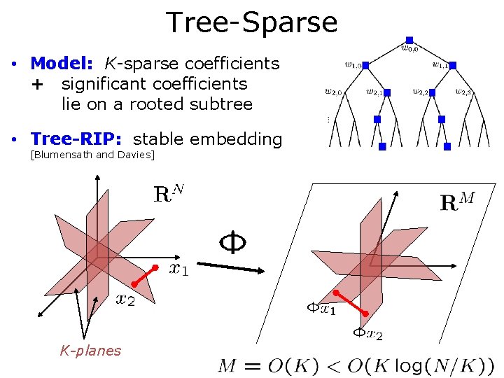
Structured-Sparse Signals • A K-sparse signal model comprises a particular (reduced) set of K-dim subspaces [Blumensath and Davies] • Fewer subspaces <> relaxed RIP <> stable recovery using fewer measurements M

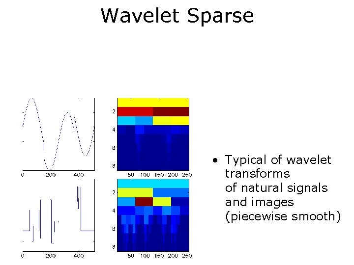
Wavelet Sparse • Typical of wavelet transforms of natural signals and images (piecewise smooth)

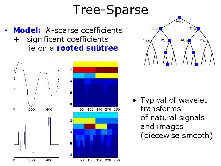
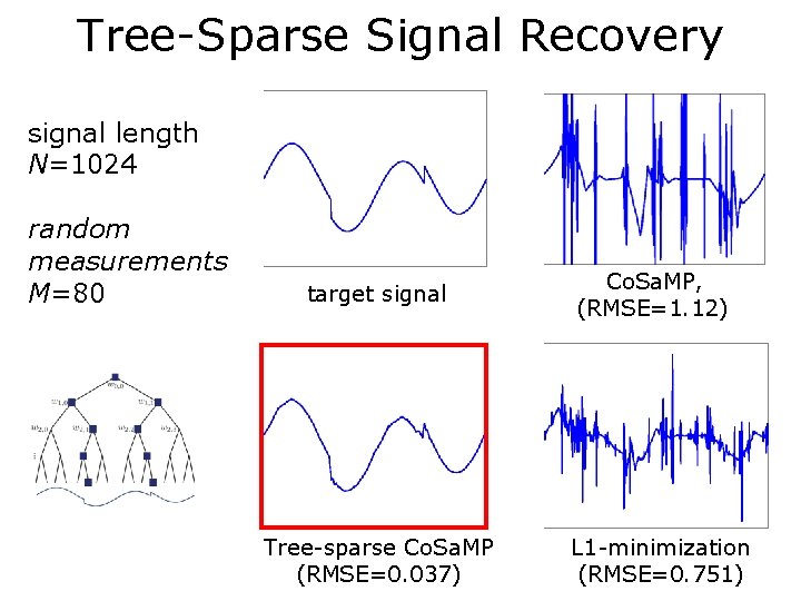
Tree-Sparse • Model: K-sparse coefficients + significant coefficients lie on a rooted subtree • Typical of wavelet transforms of natural signals and images (piecewise smooth)

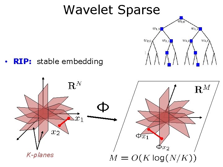
Wavelet Sparse • Model: K-sparse coefficients + significant coefficients lie on a rooted subtree • RIP: stable embedding K-planes

Tree-Sparse • Model: K-sparse coefficients + significant coefficients lie on a rooted subtree • Tree-RIP: stable embedding [Blumensath and Davies] K-planes

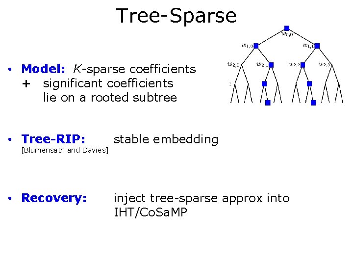
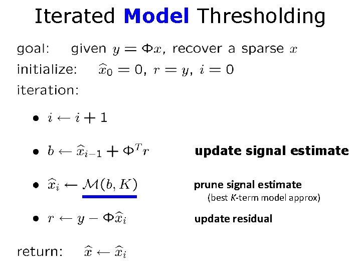
Tree-Sparse • Model: K-sparse coefficients + significant coefficients lie on a rooted subtree • Tree-RIP: stable embedding • Recovery: inject tree-sparse approx into IHT/Co. Sa. MP [Blumensath and Davies]

Recall: Iterated Thresholding update signal estimate prune signal estimate (best K-term approx) update residual

Iterated Model Thresholding update signal estimate prune signal estimate (best K-term model approx) update residual

Tree-Sparse Signal Recovery signal length N=1024 random measurements M=80 target signal Tree-sparse Co. Sa. MP (RMSE=0. 037) Co. Sa. MP, (RMSE=1. 12) L 1 -minimization (RMSE=0. 751)

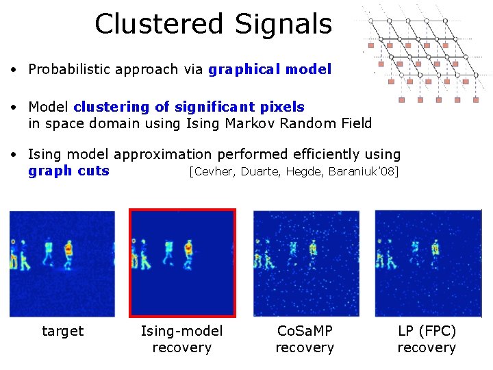
Clustered Signals • Probabilistic approach via graphical model • Model clustering of significant pixels in space domain using Ising Markov Random Field • Ising model approximation performed efficiently using graph cuts [Cevher, Duarte, Hegde, Baraniuk’ 08] target Ising-model recovery Co. Sa. MP recovery LP (FPC) recovery

Part 2: Compressive sensing Motivation, theory, recovery • Linear inverse problems • Sensing visual signals • Compressive sensing – Theory – Hallmark – Recovery algorithms • Model-based compressive sensing – Models specific to visual signals