Shop Floor Scheduling Topics to be covered 1

Shop Floor Scheduling
Topics to be covered 1. Single machine scheduling problems 2. Branch and Bound algorithm 3. Heuristics 4. Scheduling jobs on machines in series 5. Scheduling jobs on parallel machines 6. Batch scheduling 7. Assembly line balancing
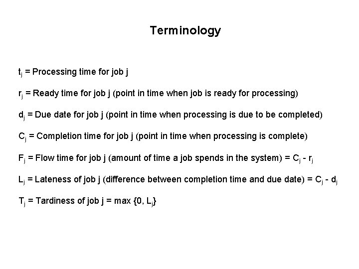
Terminology tj = Processing time for job j rj = Ready time for job j (point in time when job is ready for processing) dj = Due date for job j (point in time when processing is due to be completed) Cj = Completion time for job j (point in time when processing is complete) Fj = Flow time for job j (amount of time a job spends in the system) = Cj - rj Lj = Lateness of job j (difference between completion time and due date) = Cj - dj Tj = Tardiness of job j = max {0, Lj}
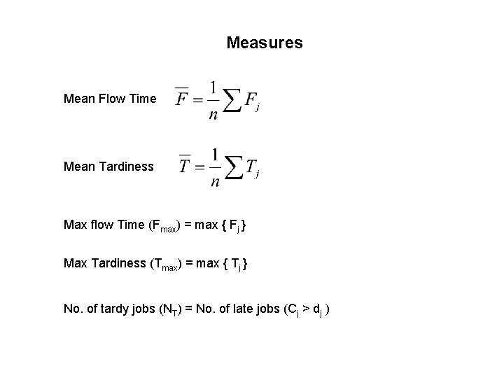
Measures Mean Flow Time Mean Tardiness Max flow Time (Fmax) = max { Fj } Max Tardiness (Tmax) = max { Tj } No. of tardy jobs (NT) = No. of late jobs (Cj > dj )

Single Machine Scheduling Problem ‘n’ jobs one machine
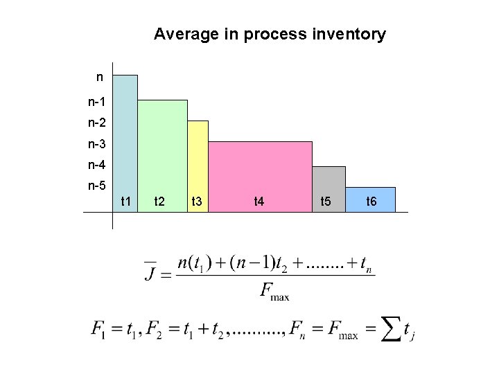
Average in process inventory n n-1 n-2 n-3 n-4 n-5 t 1 t 2 t 3 t 4 t 5 t 6
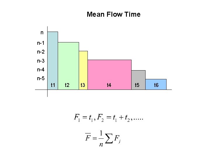
Mean Flow Time n n-1 n-2 n-3 n-4 n-5 t 1 t 2 t 3 t 4 t 5 t 6
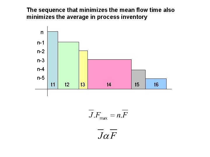
The sequence that minimizes the mean flow time also minimizes the average in process inventory n n-1 n-2 n-3 n-4 n-5 t 1 t 2 t 3 t 4 t 5 t 6
Show that, The sequence that minimizes the mean flow time also minimizes the mean completion time. The sequence that minimizes the mean flow time also minimizes the mean lateness. The sequence that minimizes the mean flow time also minimizes the mean waiting time for jobs.
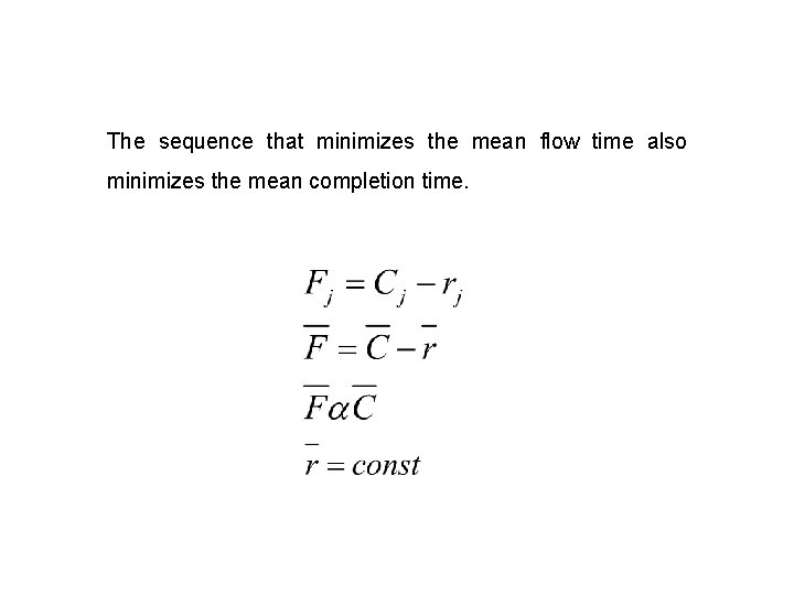
The sequence that minimizes the mean flow time also minimizes the mean completion time.
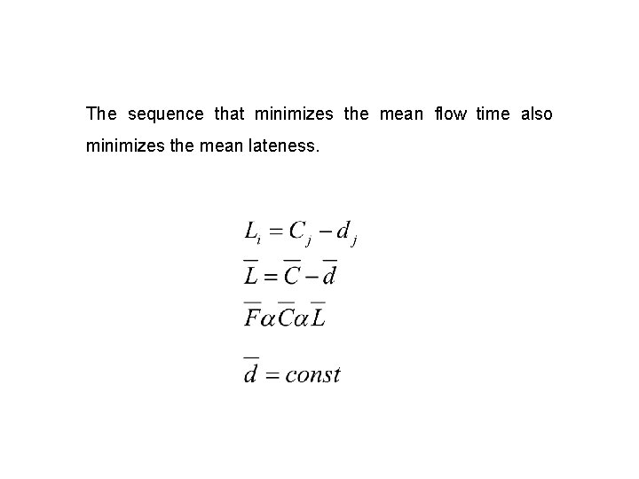
The sequence that minimizes the mean flow time also minimizes the mean lateness.
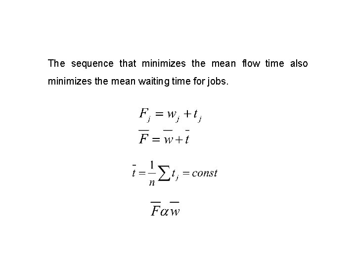
The sequence that minimizes the mean flow time also minimizes the mean waiting time for jobs.

Sequence to minimize Mean Flow Time Also check if this minimizes average w. i. p inventory
Need for heuristics Computationally, the solution to scheduling problems could be very demanding. For example, If we want to develop all possible sequences (exhaustive enumeration) for a single machine problem with ‘n’ jobs, we need to evaluate n! combinations.
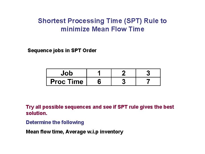
Shortest Processing Time (SPT) Rule to minimize Mean Flow Time Sequence jobs in SPT Order Try all possible sequences and see if SPT rule gives the best solution. Determine the following Mean flow time, Average w. i. p inventory
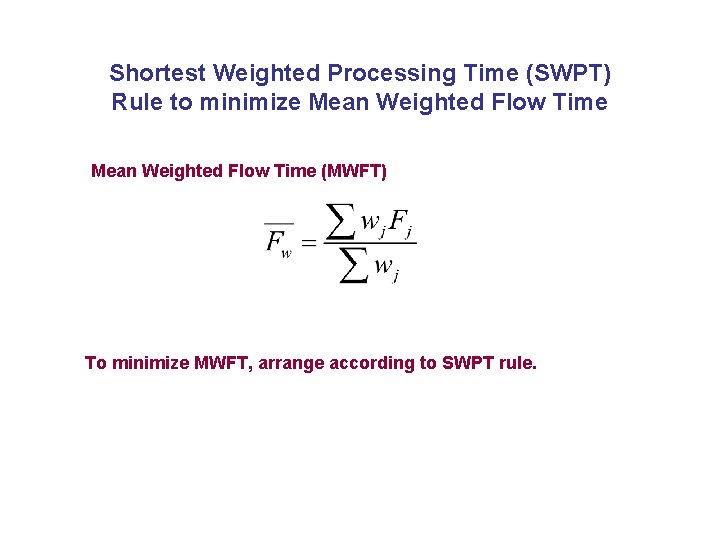
Shortest Weighted Processing Time (SWPT) Rule to minimize Mean Weighted Flow Time (MWFT) To minimize MWFT, arrange according to SWPT rule.
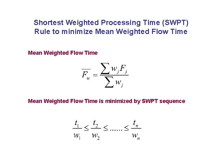
Shortest Weighted Processing Time (SWPT) Rule to minimize Mean Weighted Flow Time is minimized by SWPT sequence
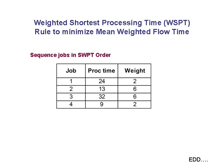
Weighted Shortest Processing Time (WSPT) Rule to minimize Mean Weighted Flow Time Sequence jobs in SWPT Order EDD….
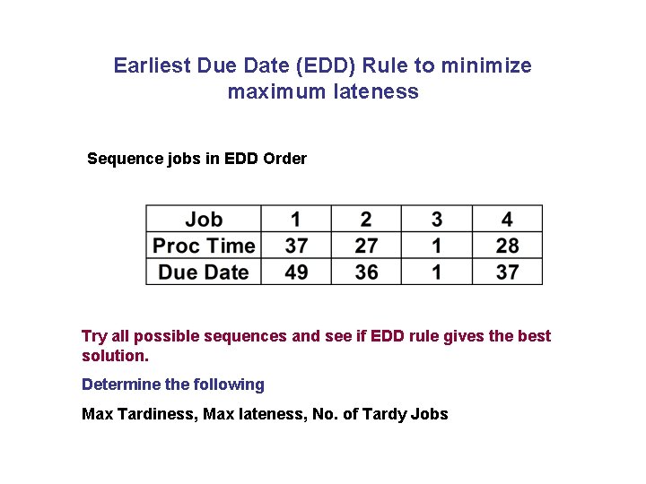
Earliest Due Date (EDD) Rule to minimize maximum lateness Sequence jobs in EDD Order Try all possible sequences and see if EDD rule gives the best solution. Determine the following Max Tardiness, Max lateness, No. of Tardy Jobs
Research findings for EDD (best solutions were known for these cases) For 5 jobs and 100 test cases, best solution was obtained approx 20% of the time for tight schedules. For 50 jobs and 100 test cases, best solution could not be was obtained even in one case for tight schedules.

Branch and Bound Algorithm
Branch and Bound Algorithm In any sequence there is always a job that is processed last, and if there are no restrictions, any job can be processed last. If the job is late, it has a penalty. The objective is to determine a sequence which leads to minimum penalty. Step 1: Draw a tree diagram indicating a node for each possible job to be processed last. Step 2: Calculate the lower bound on total penalty associated with the nodes of step 1. Total penalty is found as follows
Branch and Bound Algorithm Determine the sum of the processing time of jobs that are not yet assigned to the node in the branch including the job under consideration. Subtract the due date of the job under consideration from the above sum and multiply by the penalty. Total penalty of the jobs assigned so far is the sum of the above penalty values.
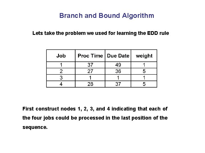
Branch and Bound Algorithm Lets take the problem we used for learning the EDD rule First construct nodes 1, 2, 3, and 4 indicating that each of the four jobs could be processed in the last position of the sequence.
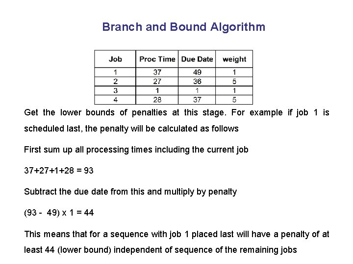
Branch and Bound Algorithm Get the lower bounds of penalties at this stage. For example if job 1 is scheduled last, the penalty will be calculated as follows First sum up all processing times including the current job 37+27+1+28 = 93 Subtract the due date from this and multiply by penalty (93 - 49) x 1 = 44 This means that for a sequence with job 1 placed last will have a penalty of at least 44 (lower bound) independent of sequence of the remaining jobs
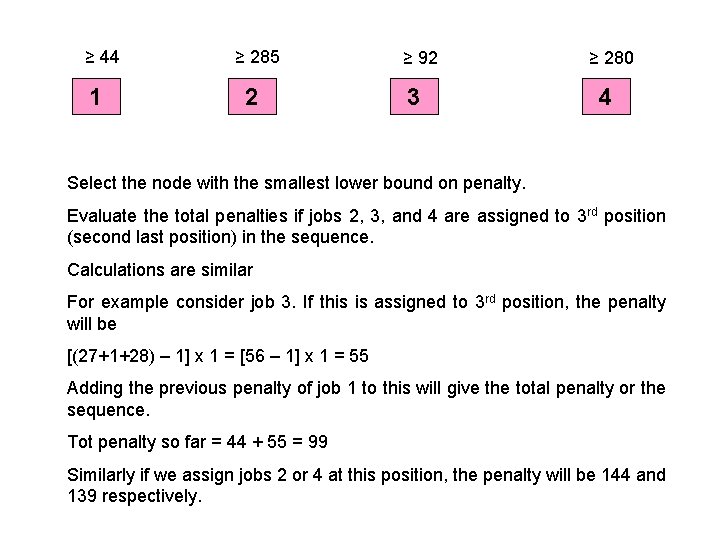
≥ 44 1 ≥ 285 2 ≥ 92 3 ≥ 280 4 Select the node with the smallest lower bound on penalty. Evaluate the total penalties if jobs 2, 3, and 4 are assigned to 3 rd position (second last position) in the sequence. Calculations are similar For example consider job 3. If this is assigned to 3 rd position, the penalty will be [(27+1+28) – 1] x 1 = [56 – 1] x 1 = 55 Adding the previous penalty of job 1 to this will give the total penalty or the sequence. Tot penalty so far = 44 + 55 = 99 Similarly if we assign jobs 2 or 4 at this position, the penalty will be 144 and 139 respectively.
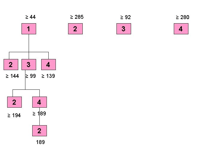
≥ 44 ≥ 285 1 2 ≥ 144 2 3 4 ≥ 99 ≥ 139 2 4 ≥ 194 ≥ 189 2 189 ≥ 92 3 ≥ 280 4
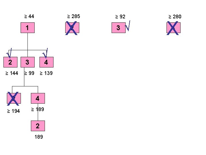
≥ 44 ≥ 285 X 1 √ 2 ≥ 144 X 2 √ 3 4 ≥ 99 ≥ 139 2 4 ≥ 194 ≥ 189 2 189 ≥ 92 3 √ ≥ 280 X 4
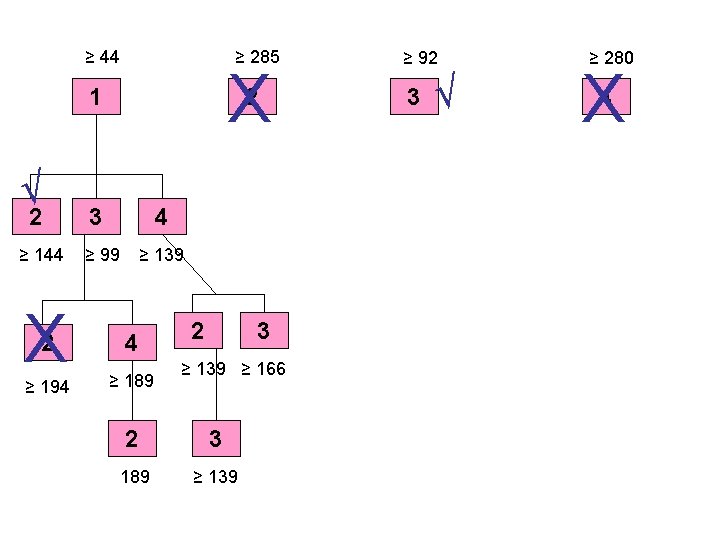
≥ 44 ≥ 285 X 1 √ 2 ≥ 144 X 2 3 4 ≥ 99 ≥ 139 2 4 ≥ 194 ≥ 189 2 3 ≥ 139 ≥ 166 2 3 189 ≥ 139 ≥ 92 3 √ ≥ 280 X 4
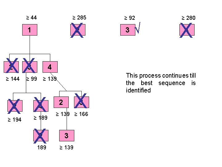
≥ 44 ≥ 285 X 1 2 XX 2 ≥ 144 3 ≥ 92 3 √ ≥ 280 X 4 4 ≥ 99 ≥ 139 X X X 2 4 ≥ 194 ≥ 189 X 2 3 ≥ 139 ≥ 166 2 3 189 ≥ 139 This process continues till the best sequence is identified
Hodgson’s Rule to minimize the number of tardy jobs Step 1: Order all jobs by EDD rule. If zero or one jobs are tardy (positive lateness), then stop. Otherwise go to step 2. Note: EDD rule minimizes maximum lateness. Therefore if the EDD sequence has zero or one tardy jobs, the solution cannot be improved by Hodgson’s heuristic.
Hodgson’s Rule to minimize the number of tardy jobs Step 2: Starting at the beginning of the EDD sequence and working toward the end, identify the first tardy job. Step 3: If the tardy job is in the ith position in the sequence, examine the first ‘i’ jobs in the sequence and identify the one with the longest processing time. Remove that job and set it aside. Revise the completion time of the other jobs to reflect the consequence of removal, and return to step 2.
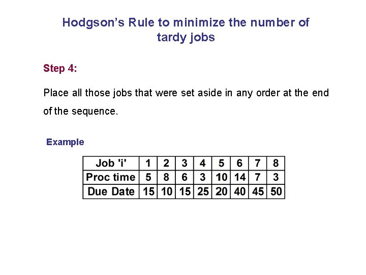
Hodgson’s Rule to minimize the number of tardy jobs Step 4: Place all those jobs that were set aside in any order at the end of the sequence. Example
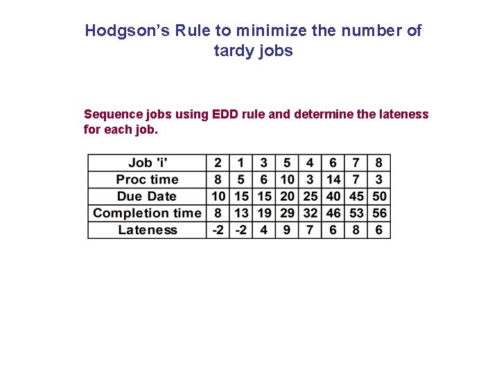
Hodgson’s Rule to minimize the number of tardy jobs Sequence jobs using EDD rule and determine the lateness for each job.
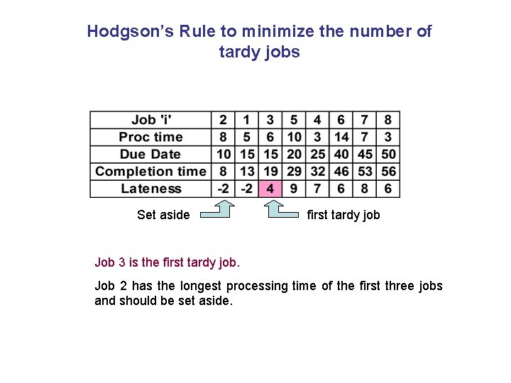
Hodgson’s Rule to minimize the number of tardy jobs Set aside first tardy job Job 3 is the first tardy job. Job 2 has the longest processing time of the first three jobs and should be set aside.
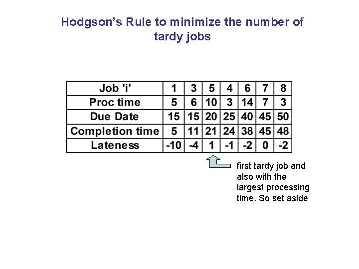
Hodgson’s Rule to minimize the number of tardy jobs first tardy job and also with the largest processing time. So set aside
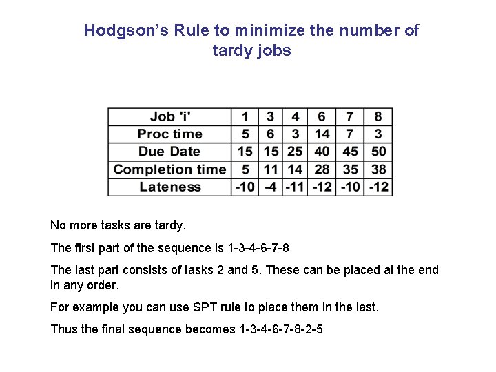
Hodgson’s Rule to minimize the number of tardy jobs No more tasks are tardy. The first part of the sequence is 1 -3 -4 -6 -7 -8 The last part consists of tasks 2 and 5. These can be placed at the end in any order. For example you can use SPT rule to place them in the last. Thus the final sequence becomes 1 -3 -4 -6 -7 -8 -2 -5
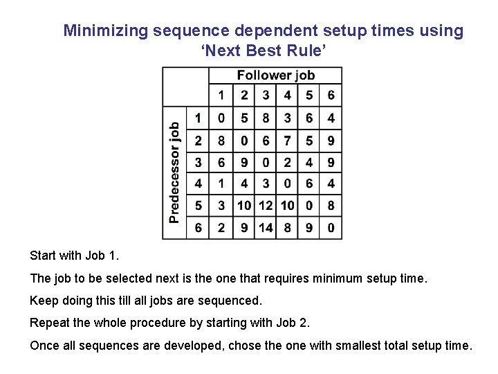
Minimizing sequence dependent setup times using ‘Next Best Rule’ Start with Job 1. The job to be selected next is the one that requires minimum setup time. Keep doing this till all jobs are sequenced. Repeat the whole procedure by starting with Job 2. Once all sequences are developed, chose the one with smallest total setup time.
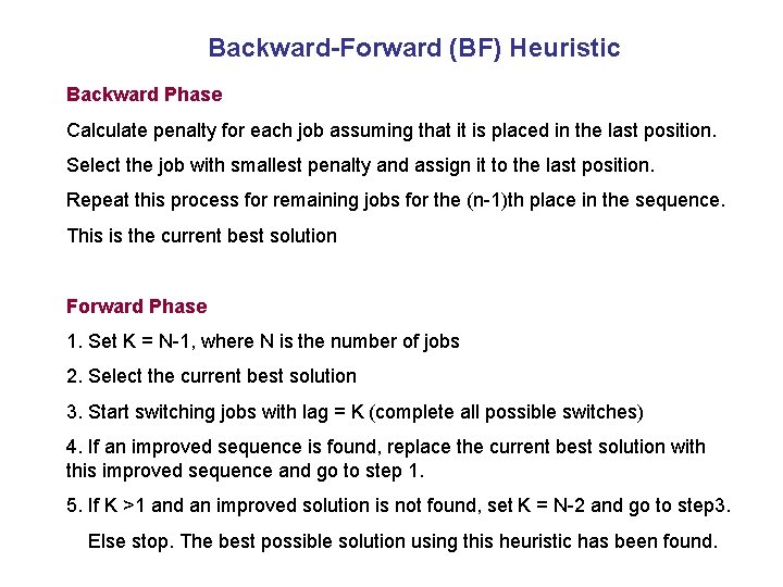
Backward-Forward (BF) Heuristic Backward Phase Calculate penalty for each job assuming that it is placed in the last position. Select the job with smallest penalty and assign it to the last position. Repeat this process for remaining jobs for the (n-1)th place in the sequence. This is the current best solution Forward Phase 1. Set K = N-1, where N is the number of jobs 2. Select the current best solution 3. Start switching jobs with lag = K (complete all possible switches) 4. If an improved sequence is found, replace the current best solution with this improved sequence and go to step 1. 5. If K >1 and an improved solution is not found, set K = N-2 and go to step 3. Else stop. The best possible solution using this heuristic has been found.
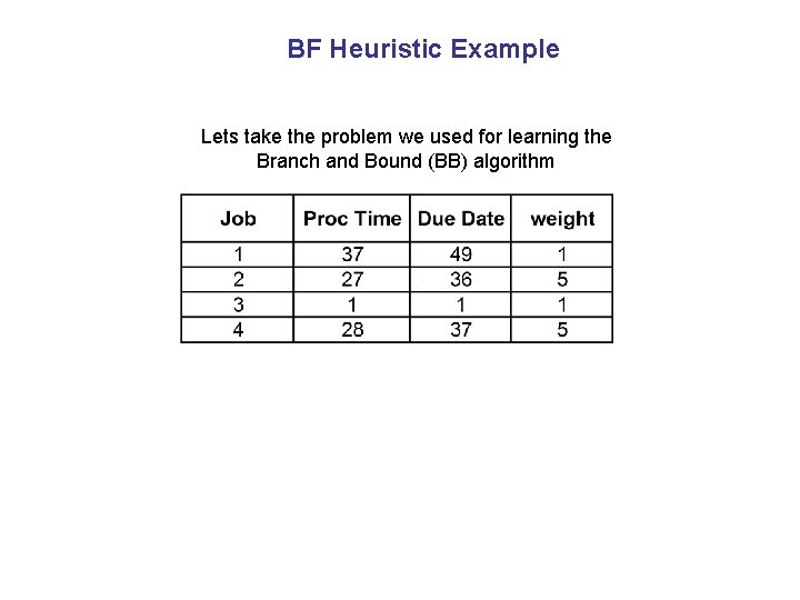
BF Heuristic Example Lets take the problem we used for learning the Branch and Bound (BB) algorithm
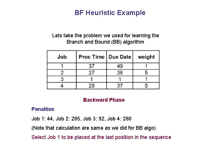
BF Heuristic Example Lets take the problem we used for learning the Branch and Bound (BB) algorithm Backward Phase Penalties Job 1: 44, Job 2: 285, Job 3: 92, Job 4: 280 (Note that calculation are same as we did for BB algo) Select Job 1 to be placed at the last position in the sequence
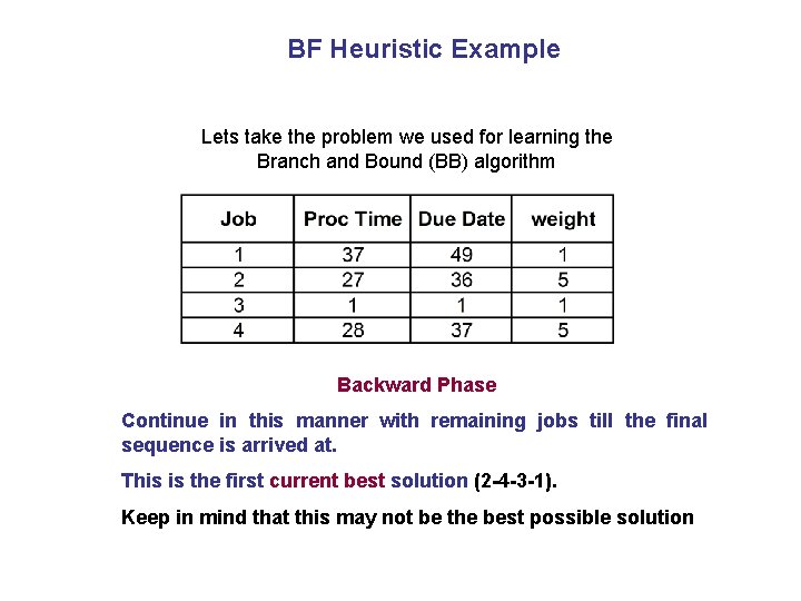
BF Heuristic Example Lets take the problem we used for learning the Branch and Bound (BB) algorithm Backward Phase Continue in this manner with remaining jobs till the final sequence is arrived at. This is the first current best solution (2 -4 -3 -1). Keep in mind that this may not be the best possible solution
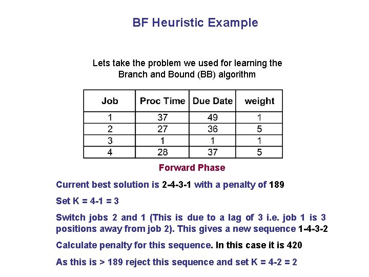
BF Heuristic Example Lets take the problem we used for learning the Branch and Bound (BB) algorithm Forward Phase Current best solution is 2 -4 -3 -1 with a penalty of 189 Set K = 4 -1 = 3 Switch jobs 2 and 1 (This is due to a lag of 3 i. e. job 1 is 3 positions away from job 2). This gives a new sequence 1 -4 -3 -2 Calculate penalty for this sequence. In this case it is 420 As this is > 189 reject this sequence and set K = 4 -2 = 2
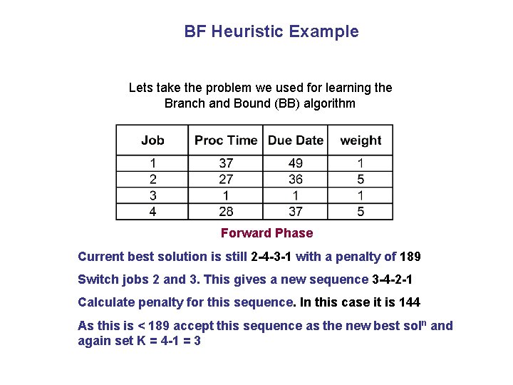
BF Heuristic Example Lets take the problem we used for learning the Branch and Bound (BB) algorithm Forward Phase Current best solution is still 2 -4 -3 -1 with a penalty of 189 Switch jobs 2 and 3. This gives a new sequence 3 -4 -2 -1 Calculate penalty for this sequence. In this case it is 144 As this is < 189 accept this sequence as the new best soln and again set K = 4 -1 = 3
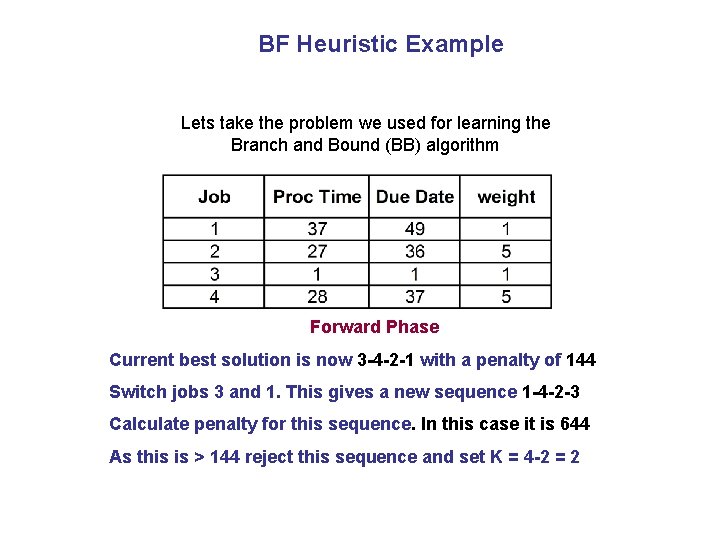
BF Heuristic Example Lets take the problem we used for learning the Branch and Bound (BB) algorithm Forward Phase Current best solution is now 3 -4 -2 -1 with a penalty of 144 Switch jobs 3 and 1. This gives a new sequence 1 -4 -2 -3 Calculate penalty for this sequence. In this case it is 644 As this is > 144 reject this sequence and set K = 4 -2 = 2
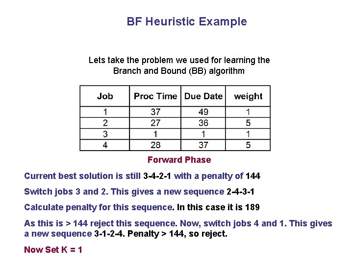
BF Heuristic Example Lets take the problem we used for learning the Branch and Bound (BB) algorithm Forward Phase Current best solution is still 3 -4 -2 -1 with a penalty of 144 Switch jobs 3 and 2. This gives a new sequence 2 -4 -3 -1 Calculate penalty for this sequence. In this case it is 189 As this is > 144 reject this sequence. Now, switch jobs 4 and 1. This gives a new sequence 3 -1 -2 -4. Penalty > 144, so reject. Now Set K = 1
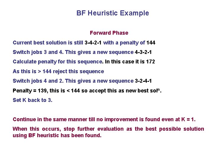
BF Heuristic Example Forward Phase Current best solution is still 3 -4 -2 -1 with a penalty of 144 Switch jobs 3 and 4. This gives a new sequence 4 -3 -2 -1 Calculate penalty for this sequence. In this case it is 172 As this is > 144 reject this sequence Switch jobs 4 and 2. This gives a new sequence 3 -2 -4 -1 Penalty = 139, this is < 144 so accept this as new best soln. Set K back to 3. Continue in the same manner till no improvement is found even at K = 1. When this occurs, stop further evaluation as the best possible solution using BF heuristic has been found.
Early and Late Penalties Motivation comes from JIT Earliness penalty can be considered as holding costs, deterioration costs etc. Tardiness penalty comes from backlogging costs, performance penalties, lost sales and goodwill
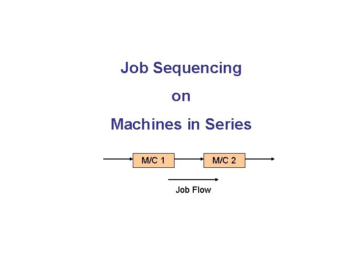
Job Sequencing on Machines in Series M/C 1 M/C 2 Job Flow
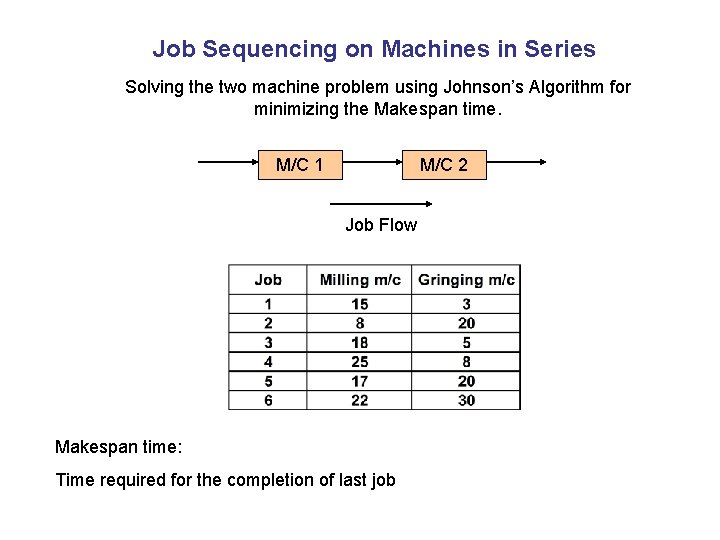
Job Sequencing on Machines in Series Solving the two machine problem using Johnson’s Algorithm for minimizing the Makespan time. M/C 1 M/C 2 Job Flow Makespan time: Time required for the completion of last job
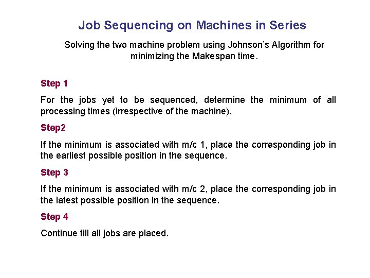
Job Sequencing on Machines in Series Solving the two machine problem using Johnson’s Algorithm for minimizing the Makespan time. Step 1 For the jobs yet to be sequenced, determine the minimum of all processing times (irrespective of the machine). Step 2 If the minimum is associated with m/c 1, place the corresponding job in the earliest possible position in the sequence. Step 3 If the minimum is associated with m/c 2, place the corresponding job in the latest possible position in the sequence. Step 4 Continue till all jobs are placed.
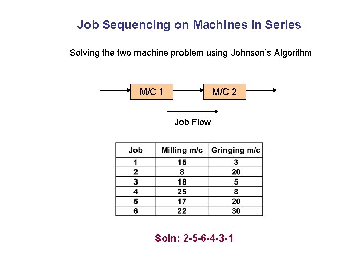
Job Sequencing on Machines in Series Solving the two machine problem using Johnson’s Algorithm M/C 1 M/C 2 Job Flow Soln: 2 -5 -6 -4 -3 -1
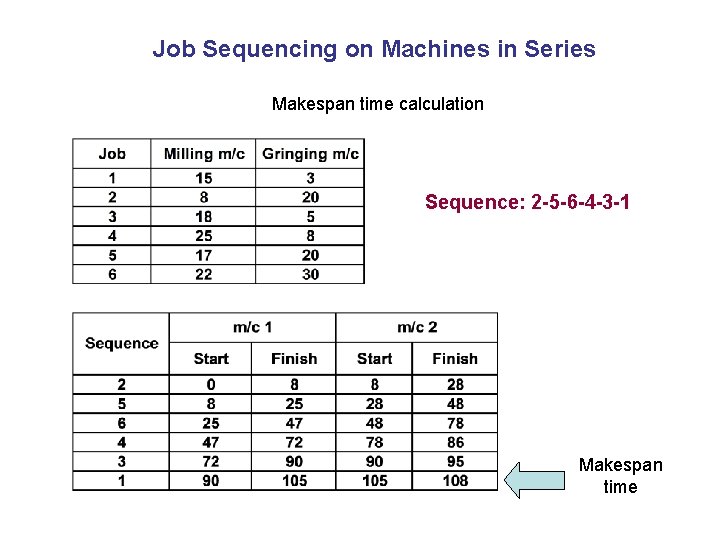
Job Sequencing on Machines in Series Makespan time calculation Sequence: 2 -5 -6 -4 -3 -1 Makespan time
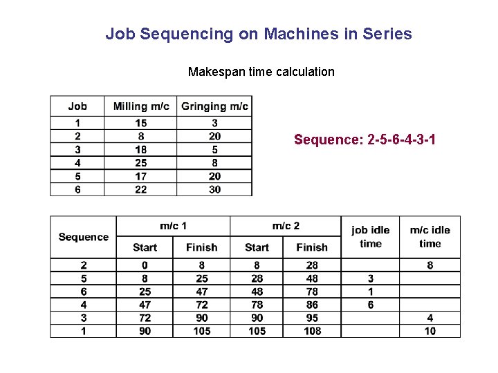
Job Sequencing on Machines in Series Makespan time calculation Sequence: 2 -5 -6 -4 -3 -1
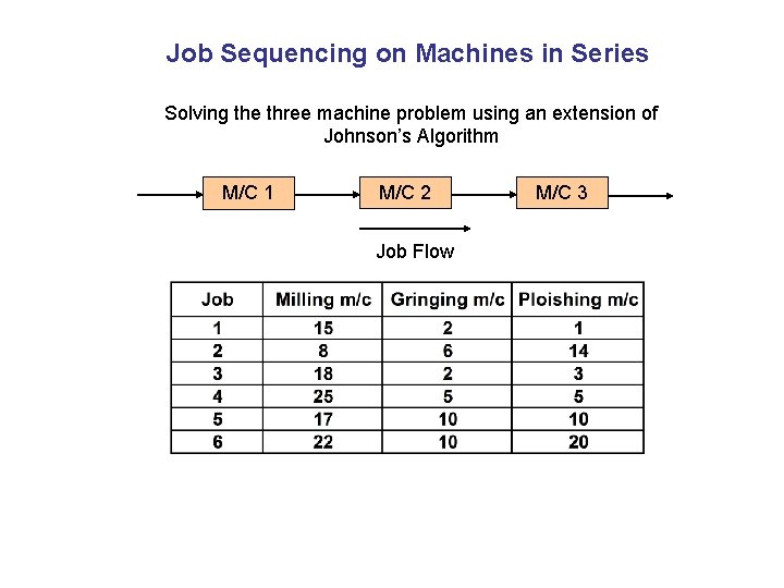
Job Sequencing on Machines in Series Solving the three machine problem using an extension of Johnson’s Algorithm M/C 1 M/C 2 Job Flow M/C 3
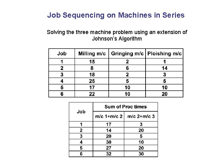
Job Sequencing on Machines in Series Solving the three machine problem using an extension of Johnson’s Algorithm
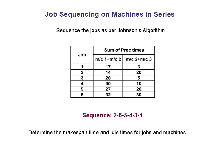
Job Sequencing on Machines in Series Sequence the jobs as per Johnson’s Algorithm Sequence: 2 -6 -5 -4 -3 -1 Determine the makespan time and idle times for jobs and machines

Sequencing ‘n’ jobs on ‘m’ Machines in Series (Algo 1)
Sequencing ‘n’ jobs on ‘m’ Machines in Series Campbell, Dudek and Smith (CDS) Heuristic 1. Set K=1 2. Schedule tasks using Johnson’s algorithm with current value of ‘K’. 3. Record the best sequence 4. Set K=K+1 5. If K=m, stop. Else, go to step 2
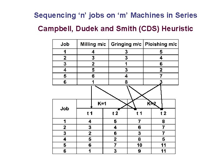
Sequencing ‘n’ jobs on ‘m’ Machines in Series Campbell, Dudek and Smith (CDS) Heuristic
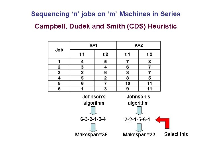
Sequencing ‘n’ jobs on ‘m’ Machines in Series Campbell, Dudek and Smith (CDS) Heuristic Johnson’s algorithm 6 -3 -2 -1 -5 -4 3 -2 -1 -5 -6 -4 Makespan=36 Makespan=33 Select this

Sequencing ‘n’ jobs on ‘m’ Machines in Series (Algo 2)
Sequencing ‘n’ jobs on ‘m’ Machines in Series Heuristic to Minimize Machine Idle Times Step 1: Find the sum of processing times for each job. Arrange the jobs in the ascending order of their sum. Schedule the job with minimum sum in the first position and calculate its completion time on each machine. Step 2: Select three jobs, if available (number can vary depending on the user), with the next minimum sum of processing times. Calculate the completion times of each job as if each job is the next one to be scheduled. Step 3: Calculate the total machine idle for each of these jobs. Step 4: The next job to be put in sequence is the one with minimum total idle time. If there is a tie, each schedule with the tied jobs may be evaluated
Sequencing ‘n’ jobs on ‘m’ Machines in Series Heuristic to Minimize Machine Idle Times Step 5: If all jobs are scheduled, stop. If not, calculate completion times for the job added to the schedule in Step 4 and go back to Step 2.
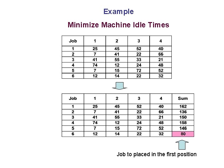
Example Minimize Machine Idle Times Job to placed in the first position
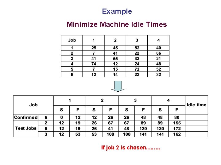
Example Minimize Machine Idle Times If job 2 is chosen……. .
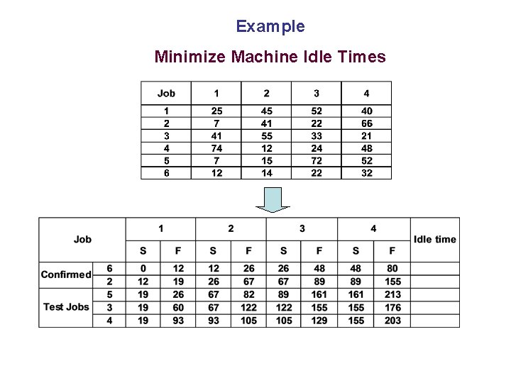
Example Minimize Machine Idle Times
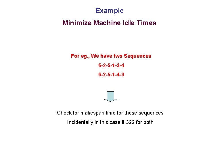
Example Minimize Machine Idle Times For eg. , We have two Sequences 6 -2 -5 -1 -3 -4 6 -2 -5 -1 -4 -3 Check for makespan time for these sequences Incidentally in this case it 322 for both

Sequencing ‘n’ jobs on ‘m’ Parallel Identical Machines
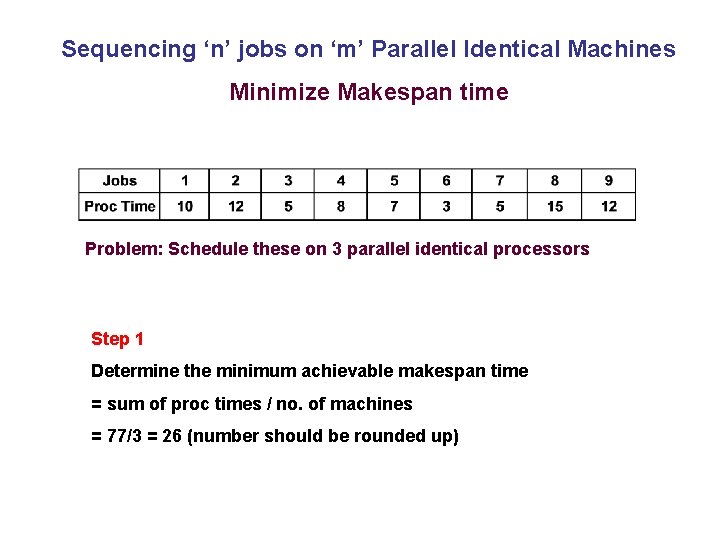
Sequencing ‘n’ jobs on ‘m’ Parallel Identical Machines Minimize Makespan time Problem: Schedule these on 3 parallel identical processors Step 1 Determine the minimum achievable makespan time = sum of proc times / no. of machines = 77/3 = 26 (number should be rounded up)
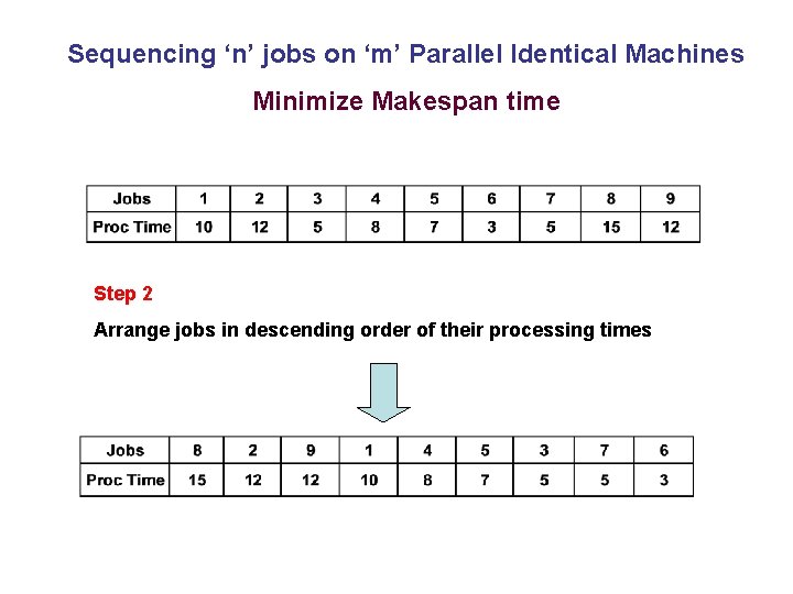
Sequencing ‘n’ jobs on ‘m’ Parallel Identical Machines Minimize Makespan time Step 2 Arrange jobs in descending order of their processing times
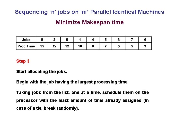
Sequencing ‘n’ jobs on ‘m’ Parallel Identical Machines Minimize Makespan time Step 3 Start allocating the jobs. Begin with the job having the largest processing time. Taking jobs from the list, one at a time, schedule them on the processor with the least amount of time already assigned (In case of a tie, break randomly).
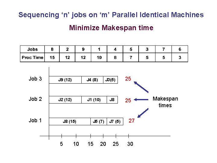
Sequencing ‘n’ jobs on ‘m’ Parallel Identical Machines Minimize Makespan time Job 3 J 9 (12) J 4 (8) Job 2 J 2 (12) J 1 (10) Job 1 J 8 (15) 5 10 J 3(5) 25 J 8 25 J 5 (7) 15 20 J 7 (5) 25 27 30 Makespan times
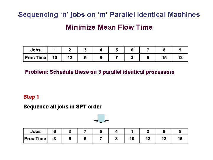
Sequencing ‘n’ jobs on ‘m’ Parallel Identical Machines Minimize Mean Flow Time Problem: Schedule these on 3 parallel identical processors Step 1 Sequence all jobs in SPT order
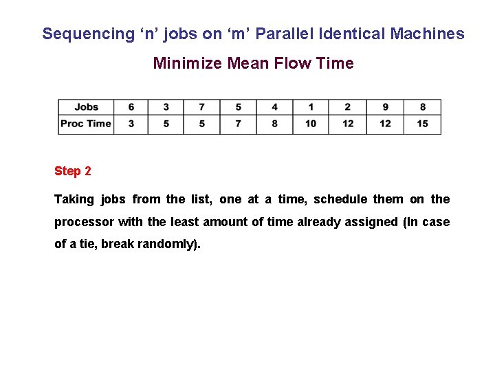
Sequencing ‘n’ jobs on ‘m’ Parallel Identical Machines Minimize Mean Flow Time Step 2 Taking jobs from the list, one at a time, schedule them on the processor with the least amount of time already assigned (In case of a tie, break randomly).
Sequencing ‘n’ jobs on ‘m’ Parallel Identical Machines Minimize Makespan and Mean flow time Step 1 Sequence all jobs in LPT (largest processing time) order Step 2 Taking jobs from the list, one at a time, schedule them on the processor with the least amount of time already assigned (In case of a tie, break randomly). Step 3 After the tasks are scheduled, order the tasks on each machine in SPT order.
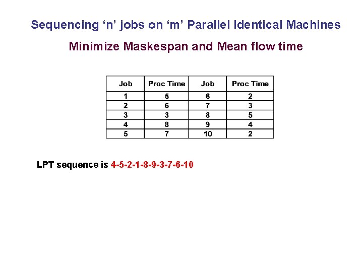
Sequencing ‘n’ jobs on ‘m’ Parallel Identical Machines Minimize Maskespan and Mean flow time LPT sequence is 4 -5 -2 -1 -8 -9 -3 -7 -6 -10
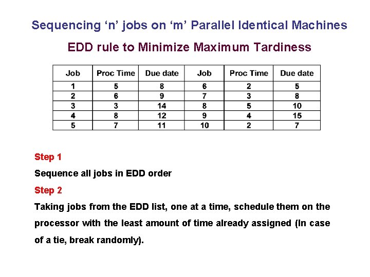
Sequencing ‘n’ jobs on ‘m’ Parallel Identical Machines EDD rule to Minimize Maximum Tardiness Step 1 Sequence all jobs in EDD order Step 2 Taking jobs from the EDD list, one at a time, schedule them on the processor with the least amount of time already assigned (In case of a tie, break randomly).
- Slides: 78