Shaqra University College of Computer and Information Sciences

Shaqra University College of Computer and Information Sciences Information Technology Department Cs 401 - Intelligent systems Chapter 3 PROBLEM SOLVING BY SEARCHING (2)

Informed Search • One that uses problem specific knowledge beyond the definition of the problem itself to guide the search. • Why? – Without incorporating knowledge into searching, one is forced to look everywhere to find the answer. Hence, the complexity of uninformed search is intractable. – With knowledge, one can search the state space as if he was given “hints” when exploring a maze. • Heuristic information in search = Hints – Leads to dramatic speed up in efficiency.

Informed Search • Best-First Search – Greedy Best First Search – A* Search • Local search algorithms • Stochastic Search algorithms

Best first search • Key idea: 1. Use an evaluation function f(n) for each node: • estimate of “distance” to the goal. 2. Node with the lowest evaluation is chosen for expansion. • Implementation: – fringe: maintain the fringe in ascending order of fvalues • Special cases: – Greedy search – A* search

Formal description of Best-First Search algorithm Function Best-First Search(problem, fringe, f) returns a solution or a failure // f: evaluation function fringe ← Insert (Make-Node(Initial-state[problem], NULL, d, c), fringe) Loop do If Empty? (fringe) then return failure node ← Remove-First (fringe) If Goal-Test[ problem] applied to State[node] succeeds then return Solution (node) fringe ← Insert-all( Expand (node, problem), fringe) sort fringe in ascending order of f-values

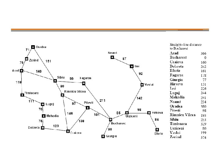
Greedy search • • – – • • • Let evaluation function f(n) be an estimate of cost from node n to goal This function is often called a heuristic and is denoted by h(n). f(n) = h(n) e. g. h. SLD(n) = straight-line distance from n to Bucharest Greedy search expands the node that appears to be closest to goal. Contrast with uniform-cost search in which lowest cost path from start is expanded. Heuristic function is the way knowledge about the problem is used to guide the search process.

Greedy search

Greedy search

Greedy search

Greedy Search Properties • Finds solution without ever expanding a node that is not on the solution path. • It is not optimal: the optimal path goes trough Ptesti. • Minimizing h(n) is susceptible to false starts. – e. g getting from Iasi to Fagaras: according to h(n), we take Neamt node to expand but it is a dead end. • If repeated states are not detected, the solution will never be found. Search gets stuck in loops: – Iasi →Neamet → Iasi → Neamet • Complete in finite spaces with repeated state checking.

A* search • Most widely known for best-first search. • Key idea: avoid expanding paths that are already expensive. • Evaluation function: f(n) = g(n) + h(n) – g(n) = path cost so far to reach n. (used in Uniform Cost Search). – h(n) = estimated path cost to goal from n. (used in Greedy Search). – f(n) = estimated total cost of path through n to goal.

A* search

A* search

A* search

A* search

A* search

A* search • Definition: a heuristic h(n) is said to be admissible if it never overestimates the cost to reach the goal. h(n) h*(n) • where h*(n) is the TRUE cost from n. • e. g: hsld straight line can not be an overestimate. • Consequently: if h(n) is an admissible heuristic, then f(n) never overestimates the true cost of a solution through n. WHY? • It is true because g(n) gives the exact cost to reach n.

A* search root g(n): cost of path n h*(n): true minimum cost to goal h(n): Heuristic (expected) minimum cost to goal. (estimation) Goal

A* search • Theorem: When Tree-Search is used, A* is optimal if h(n) is an admissible heuristic. • Proof: – Let G be the optimal goal state reached by a path with cost : C* =f(G) = g(G). – Let G 2 be some other goal state or the same state, but reached by a more costly path.

A* search f(G 2) = g(G 2)+h(G 2) = g(G 2) since h(G 2) = 0 g(G 2) > C* since G 2 is suboptimal • Let n be any unexpanded node on the shortest path to the optimal goal G. f(n) = g(n) + h(n) ≤ C* since h is admissible Therefore, f(n) ≤ C* ≤ f(G 2) • As a consequence, G 2 will not be expanded and A* must return an optimal solution.

A* search • • Consistency (= Monotonicity): A heuristic is said to be consistent when for any node n, successor n’ of n, we have h(n) ≤ c(n, n’) + h(n’), where c(n, n’) is the (minimum) cost of a step from n to n’. This is a form of triangular inequality: h(n) n c(n, n’) g h(n’) n’ • • • Consistent heuristics are admissible. Not all admissible heuristics are consistent. When a heuristic is consistent, the values of f(n) along any path are nondecreasing. A* with a consistent heuristic is optimal.

A* search properties • Completeness: Yes, unless there are infinitely many nodes with f ≤ f(G). • Optimality: Yes. • Time: Exponential. • Space: Keeps all nodes in memory.

Some admissible heuristics • 8 -Puzzle: – g(n): the path cost can be measured by the total number of horizontal and vertical moves. – h(n): two different heuristics – h 1 (n): number of misplaced tiles. – h 2 (n): the sum of the distances of the tiles from their goal positions.

Local Search algorithms • The search algorithms we have seen so far keep track of the current state, the “fringe” of the search space, and the path to the final state. • In some problems, one doesn’t care about a solution path but only the final goal state. The solution is the goal state. Example: 8 -queen problem. • Local search algorithms are also useful for optimization problems where the goal is to find a state such that an objective function is optimized. • For the 8 -queen algorithm, the objective function may be the number of attacks.

Local Search algorithms • Basic idea: – Local search algorithms operate on a single state – current state – and move to one of its neighboring states. – Therefore: Solution path needs not be maintained. – Hence, the search is “local”. • Two advantages: 1. Use little memory. 2. More applicable in searching large/infinite search space. They find reasonable solutions in this case.

Local Search algorithms • A state space landscape is a graph of states associated with their costs • Problem: local search can get stuck on a local maximum and not find the optimal solution

Hill Climbing • Hill climbing search algorithm (also known as greedy local search) uses a loop that continually moves in the direction of increasing values (that is uphill). • It terminates when it reaches a peak where no neighbor has a higher value. • A complete local search algorithm always find a goal if one exists. • An optimal algorithm always finds a global maximum/minimum.

Steepest ascent version Function Hill climbing (problem) return state that is a local maximum Inputs: problem, a problem Local variables: current, a node neighbor, a node Current ← Make-Node (initial-state [problem]) Loop do neighbor ← a highest-valued successor of current If Value[neighbor] ≤ Value[current] then return state [current] Current ← neighbor

Simulated Annealing • Basic inspiration: What is annealing? • In mettallurgy, annealing is the physical process used to temper or harden metals or glass by heating them to a high temperature and then gradually cooling them, thus allowing the material to coalesce into a low energy cristalline state. • Heating then slowly cooling a substance to obtain a strong cristalline structure. • Key idea: Simulated Annealing combines Hill Climbing with a random walk in some way that yields both efficiency and completeness. • Used to solve VLSI layout problems in the early 1980.

Simulated Annealing

Simulated Annealing Function Simulated annealing (problem, schedule) return a solution state Inputs: problem, a problem schedule, a mapping from time to temperature Local variables: current, a node next, a node T, a temperature controlling the probability of downward steps Current ← Make-Node (initial-state [problem]) For t← 1 to ∞ do T ← schedule [t] If T=0 then return current Loop do Next ← a randomly selected successor of current. ∆E ← Value [next] - Value [current] If ∆E > 0 then current ← next Else current ← next only with probability e -∆E/k. T

Local Beam Search • Unlike Hill Climbing, Local Beam Search keeps track of k states rather than just one. • It starts with k randomly generated states. • At each step, all the successors of all the states are generated. • If any one is a goal, the algorithm halts, otherwise it selects the k best successors from the complete list and repeats. • LBS≠ running k random restarts in parallel instead of sequence. • Drawback: less diversity → Stochastic Beam Search

Stochastic search: Genetic algorithms • Formally introduced in the US in the 70 s by John Holland. • GAs emulate ideas from genetics and natural selection and can search potentially large spaces. • Before we can apply Genetic Algorithm to a problem, we need to answer: – – How is an individual represented What is the fitness function? How are individuals selected? How do individuals reproduce?

Stochastic search: Genetic algorithms • Genetic algorithms is a variant of local beam search. • Successors in this case are generated by combining two parent states rather than modifying a single state. • Like local beam search, genetic algorithms starts with a set of k randomly generated states called Population. • Each state or individual is represented as a string over a finite alphabet. It is also called chromosome.

Stochastic search: Genetic algorithms • Each state is rated by the evaluation function called fitness function. • Fitness function should return higher values for better states. • For reproduction, individuals are selected with a probability which is directly proportional to the fitness score. • For each pair to be mated, a crossover point is randomly chosen from the positions in the string. • The offsprings themselves are created by crossing over the parent strings at the crossover point. • Mutation is performed randomly with a small independent probability.

Stochastic search: Genetic algorithms

Stochastic search: Genetic algorithms Function Genetic-Algorithm (population, fitness-Fn) returns individual Inputs: population, a set of individuals fitness-Fn, a function that measures the fitness of an individual Repeat New population ← empty set; for i from 1 to Size. Population do {x ← random-Selection (population, fitness-Fn); y ← random-Selection (population, fitness-Fn); Child ← Reproduce (x, y); If (small random probability) then child ← mutate(child) Add child to new population } Population ← new population Until some individual is fit enough or enough time has elapsed; Return the best individual in population, according to Fitness-Fn

Summary • Informed search uses knowledge about the problem to reduce search costs. • This knowledge is expressed in terms of heuristics. • Best first search is a class of methods that use a variant of graph-search where the minimum-cost unexpanded nodes are chosen for expansion. • Best first search methods use a heuristic function h(n) that estimates the cost of a solution from a node. • Greedy search is a best first search that expands nodes with minimal h(n). It is not optimal but often efficient. • A* search is a best first search that takes into account the total cost from the root node to goal node. It expands node with minimal f(n) = g(n) + h(n). It is complete and optimal provided that h(n) is admissible (for tree search) or consistent (for graph search). The space complexity is prohibitive.

Summary • Construction of heuristics can be done by relaxing the problem definition (in a sense simplifying the problem), by precomputing solution costs for subproblems or learning from experience with the problem class. • Local search methods keep small number of nodes in memory. They are suitable for problems where the solution is the goal state itself and not the path. • Hill climbing, simulated annealing and local beam search are examples of local search algorithms. • Stochastic algorithms represent another class of methods for informed search. Genetic algorithms are a kind of stochastic hill-climbing search in which a large population of states is maintained. New states are generated by mutation and by crossover which combines pairs of states from the population.