Shape Analysis and Retrieval Statistical Shape Descriptors Notes

Shape Analysis and Retrieval Statistical Shape Descriptors Notes courtesy of Funk et al. , SIGGRAPH 2004

Outline: • Shape Descriptors • Statistical Shape Descriptors • Singular Value Decomposition (SVD)

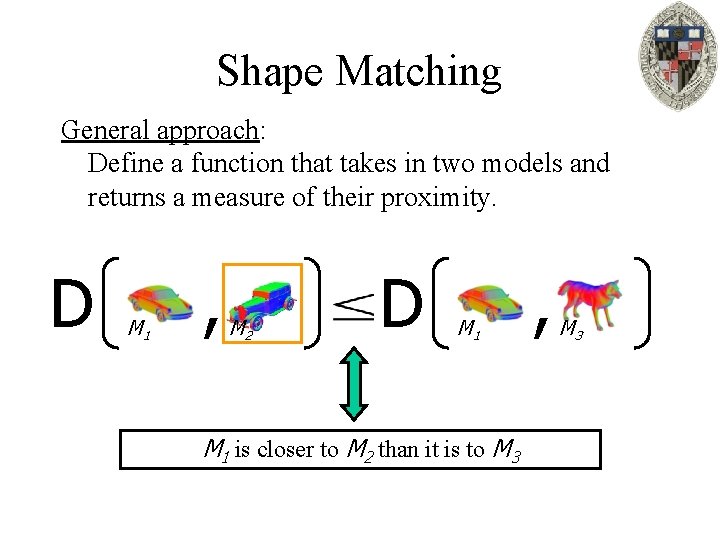
Shape Matching General approach: Define a function that takes in two models and returns a measure of their proximity. D M 1 , M 2 D M 1 is closer to M 2 than it is to M 3 , M 3

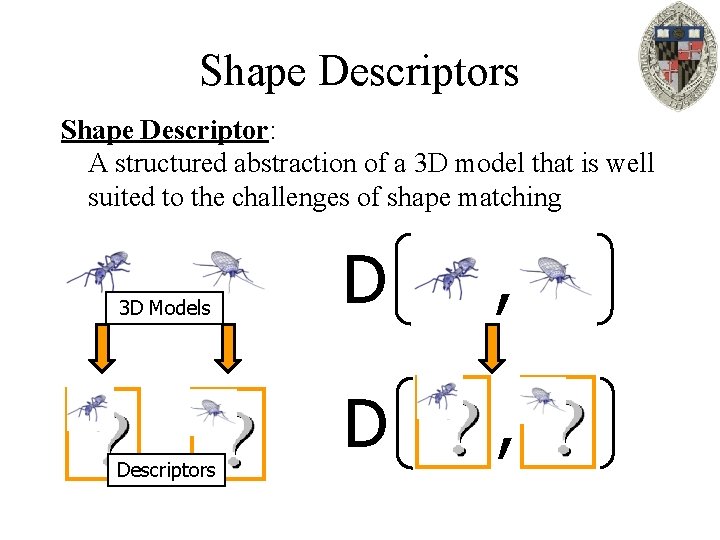
Shape Descriptors Shape Descriptor: A structured abstraction of a 3 D model that is well suited to the challenges of shape matching 3 D Models Descriptors D ,

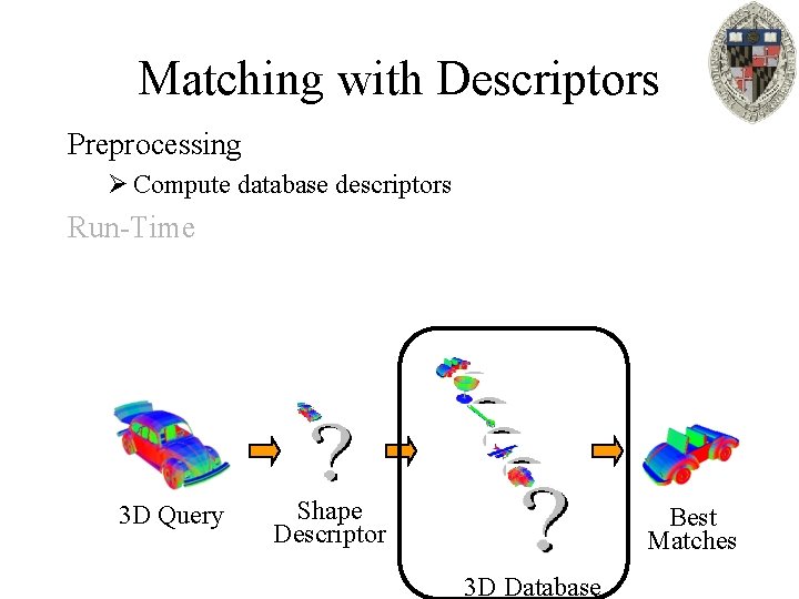
Matching with Descriptors Preprocessing Ø Compute database descriptors Run-Time 3 D Query Shape Descriptor Best Matches 3 D Database

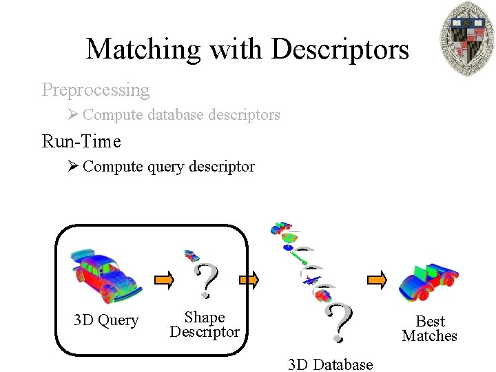
Matching with Descriptors Preprocessing Ø Compute database descriptors Run-Time Ø Compute query descriptor 3 D Query Shape Descriptor Best Matches 3 D Database

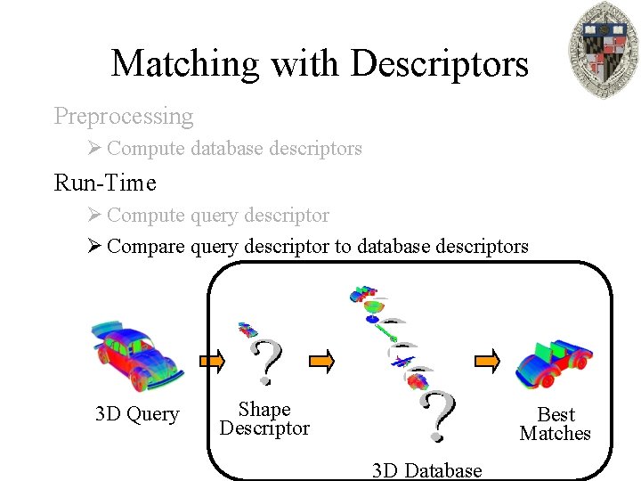
Matching with Descriptors Preprocessing Ø Compute database descriptors Run-Time Ø Compute query descriptor Ø Compare query descriptor to database descriptors 3 D Query Shape Descriptor Best Matches 3 D Database

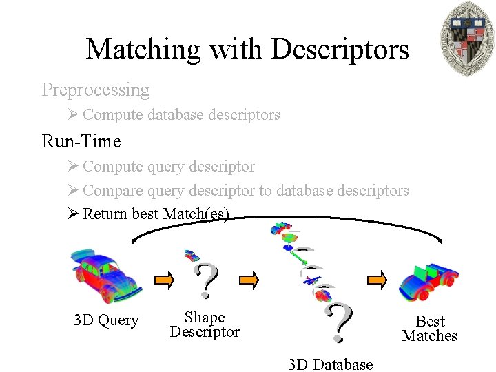
Matching with Descriptors Preprocessing Ø Compute database descriptors Run-Time Ø Compute query descriptor Ø Compare query descriptor to database descriptors Ø Return best Match(es) 3 D Query Shape Descriptor Best Matches 3 D Database

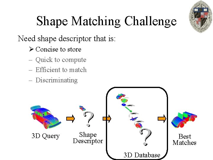
Shape Matching Challenge Need shape descriptor that is: Ø Concise to store – Quick to compute – Efficient to match – Discriminating 3 D Query Shape Descriptor Best Matches 3 D Database

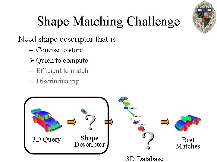
Shape Matching Challenge Need shape descriptor that is: – Concise to store Ø Quick to compute – Efficient to match – Discriminating 3 D Query Shape Descriptor Best Matches 3 D Database

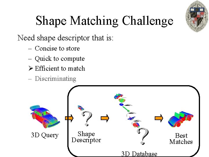
Shape Matching Challenge Need shape descriptor that is: – Concise to store – Quick to compute Ø Efficient to match – Discriminating 3 D Query Shape Descriptor Best Matches 3 D Database

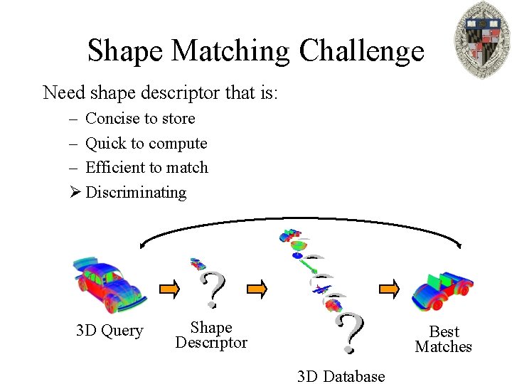
Shape Matching Challenge Need shape descriptor that is: – Concise to store – Quick to compute – Efficient to match Ø Discriminating 3 D Query Shape Descriptor Best Matches 3 D Database

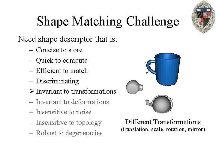
Shape Matching Challenge Need shape descriptor that is: – Concise to store – Quick to compute – Efficient to match – Discriminating Ø Invariant to transformations – Invariant to deformations – Insensitive to noise Different Transformations – Insensitive to topology (translation, scale, rotation, mirror) – Robust to degeneracies

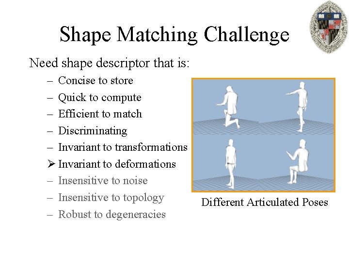
Shape Matching Challenge Need shape descriptor that is: – Concise to store – Quick to compute – Efficient to match – Discriminating – Invariant to transformations Ø Invariant to deformations – Insensitive to noise – Insensitive to topology – Robust to degeneracies Different Articulated Poses

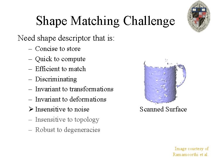
Shape Matching Challenge Need shape descriptor that is: – Concise to store – Quick to compute – Efficient to match – Discriminating – Invariant to transformations – Invariant to deformations Ø Insensitive to noise – Insensitive to topology – Robust to degeneracies Scanned Surface Image courtesy of Ramamoorthi et al.

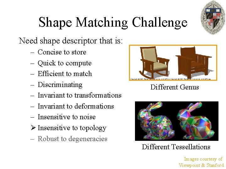
Shape Matching Challenge Need shape descriptor that is: – Concise to store – Quick to compute – Efficient to match – Discriminating – Invariant to transformations – Invariant to deformations – Insensitive to noise Ø Insensitive to topology – Robust to degeneracies Different Genus Different Tessellations Images courtesy of Viewpoint & Stanford

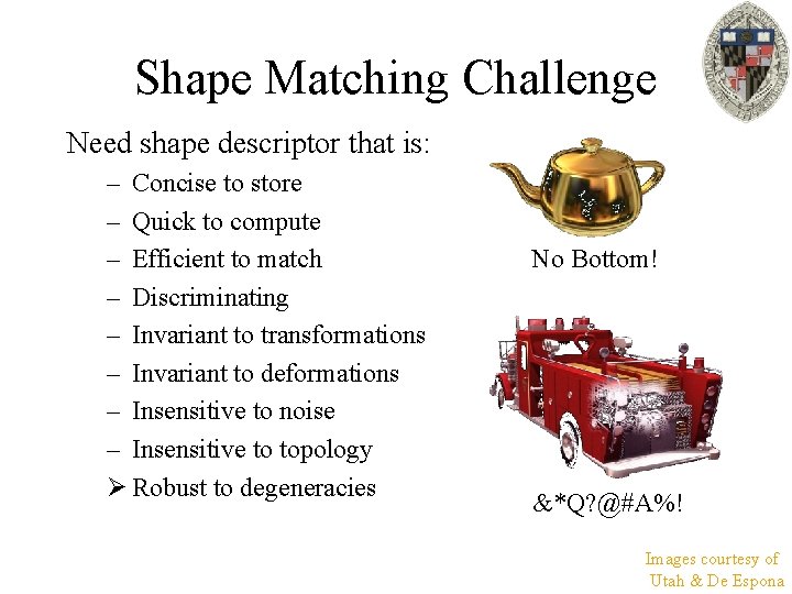
Shape Matching Challenge Need shape descriptor that is: – Concise to store – Quick to compute – Efficient to match – Discriminating – Invariant to transformations – Invariant to deformations – Insensitive to noise – Insensitive to topology Ø Robust to degeneracies No Bottom! &*Q? @#A%! Images courtesy of Utah & De Espona

Outline: • Shape Descriptors • Statistical Shape Descriptors • Singular Value Decomposition (SVD)

Statistical Shape Descriptors Challenge: Want a simple shape descriptor that is easy to compare and gives a continuous measure of the similarity between two models. Solution: Represent each model by a vector and define the distance between models as the distance between corresponding vectors.

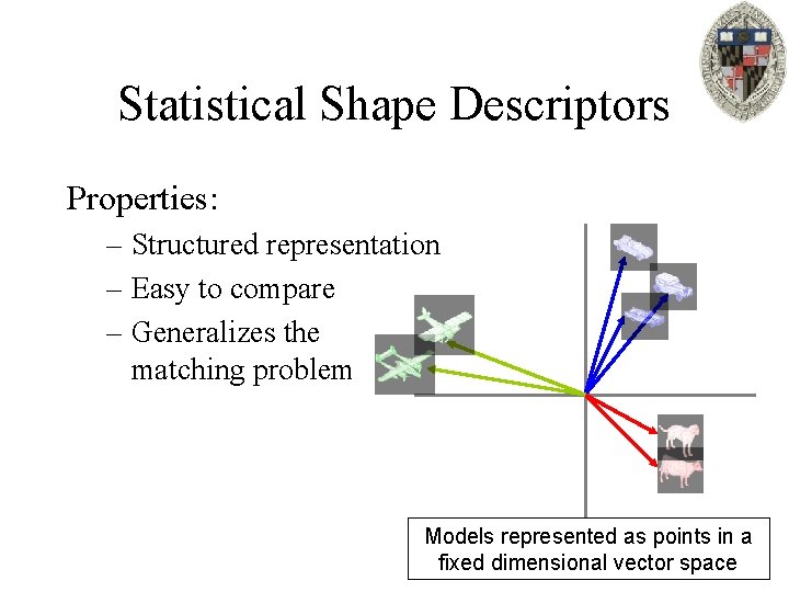
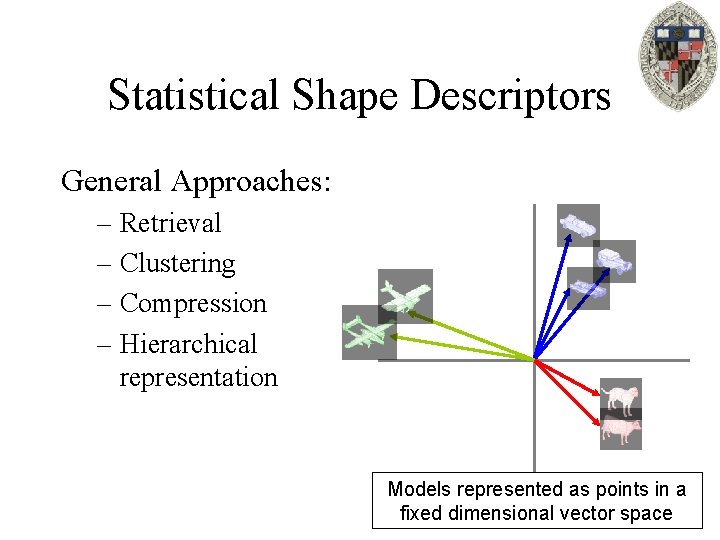
Statistical Shape Descriptors Properties: – Structured representation – Easy to compare – Generalizes the matching problem Models represented as points in a fixed dimensional vector space

Statistical Shape Descriptors General Approaches: – Retrieval – Clustering – Compression – Hierarchical representation Models represented as points in a fixed dimensional vector space

Outline: • Shape Descriptors • Statistical Shape Descriptors • Singular Value Decomposition (SVD)

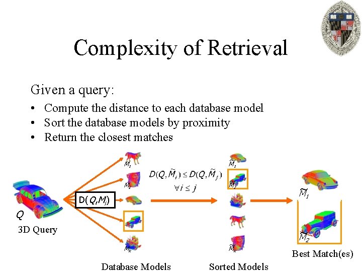
Complexity of Retrieval Given a query: • Compute the distance to each database model • Sort the database models by proximity • Return the closest matches M 1 ~1 M M 2 ~2 M D(Q, Mi) ~ M 1 Q 3 D Query Mk Database Models ~k M Sorted Models ~ M 2 Best Match(es)

Complexity of Retrieval If there are k models in the database and each model is represented by an n-dimensional vector: • Computing the distance to each database model: – O(k n) time • Sort the database models by proximity: – O(k logk) time If n is large, retrieval will be prohibitively slow.

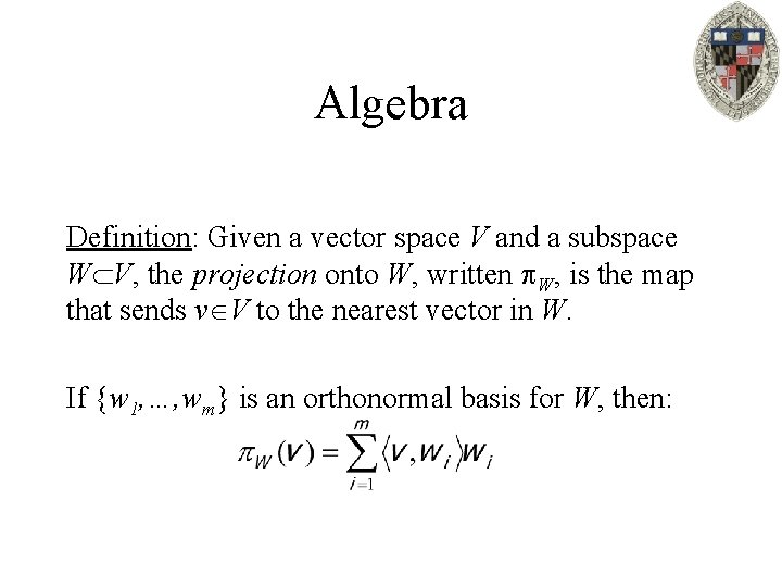
Algebra Definition: Given a vector space V and a subspace W V, the projection onto W, written W, is the map that sends v V to the nearest vector in W. If {w 1, …, wm} is an orthonormal basis for W, then:

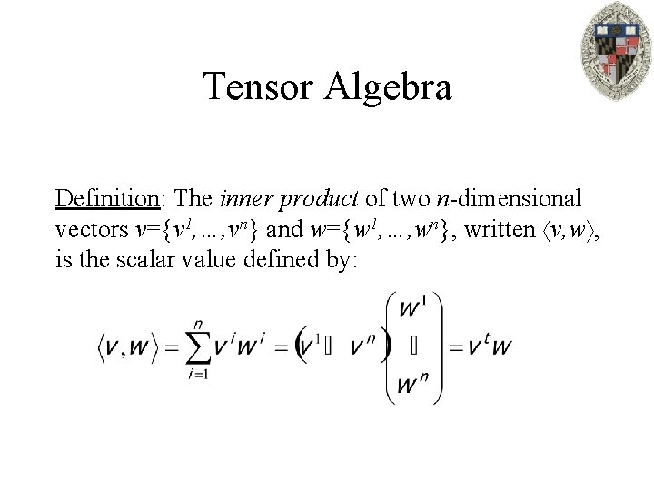
Tensor Algebra Definition: The inner product of two n-dimensional vectors v={v 1, …, vn} and w={w 1, …, wn}, written v, w , is the scalar value defined by:

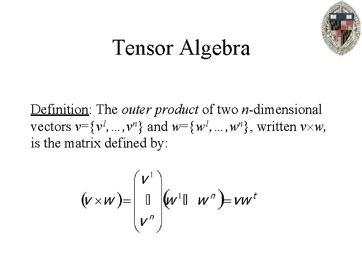
Tensor Algebra Definition: The outer product of two n-dimensional vectors v={v 1, …, vn} and w={w 1, …, wn}, written v w, is the matrix defined by:

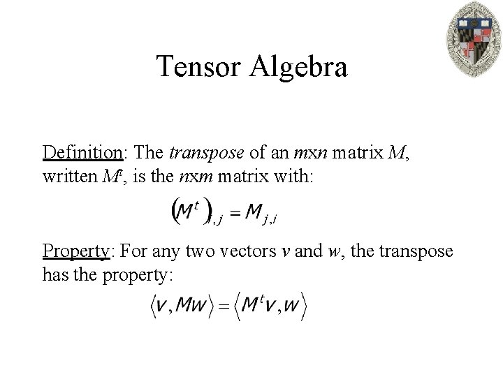
Tensor Algebra Definition: The transpose of an mxn matrix M, written Mt, is the nxm matrix with: Property: For any two vectors v and w, the transpose has the property:

SVD Compression Key Idea: Given a collection of vectors in n-dimensional space, find a good m-dimensional subspace (m<<n) in which to represent the vectors.

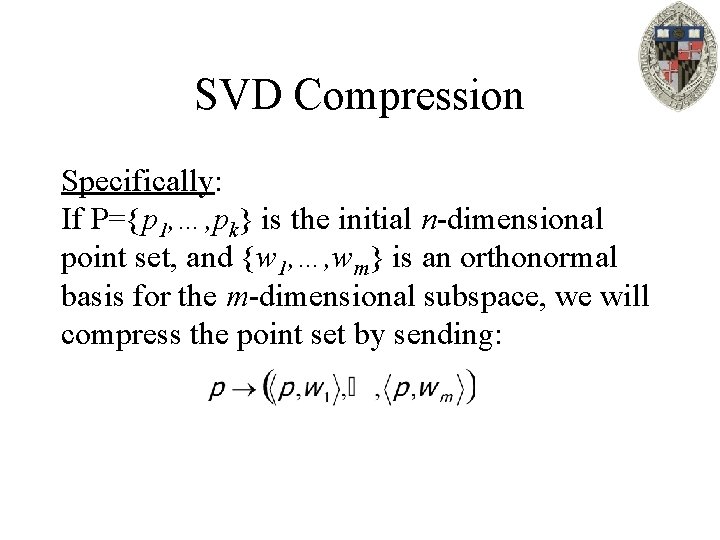
SVD Compression Specifically: If P={p 1, …, pk} is the initial n-dimensional point set, and {w 1, …, wm} is an orthonormal basis for the m-dimensional subspace, we will compress the point set by sending:

SVD Compression Challenge: To find the m-dimensional subspace that will best capture the initial point information.

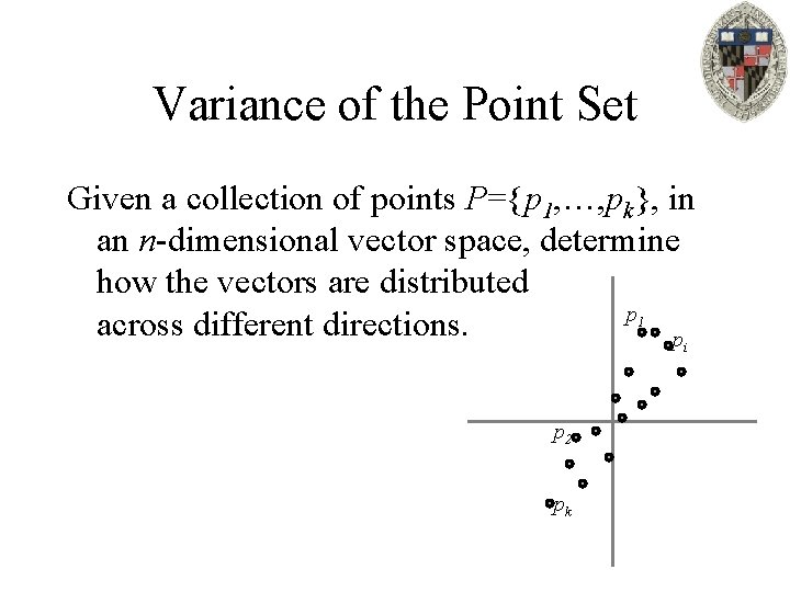
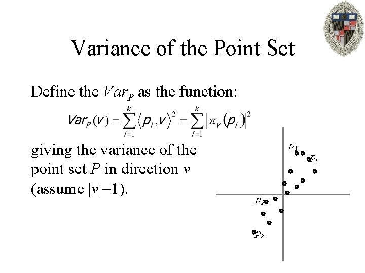
Variance of the Point Set Given a collection of points P={p 1, …, pk}, in an n-dimensional vector space, determine how the vectors are distributed p 1 across different directions. pi p 2 pk

Variance of the Point Set Define the Var. P as the function: giving the variance of the point set P in direction v (assume |v|=1). p 1 p 2 pk pi

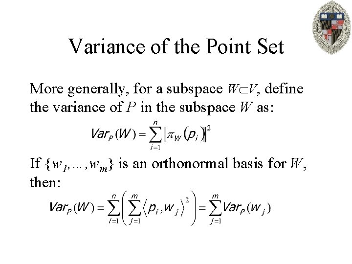
Variance of the Point Set More generally, for a subspace W V, define the variance of P in the subspace W as: If {w 1, …, wm} is an orthonormal basis for W, then:

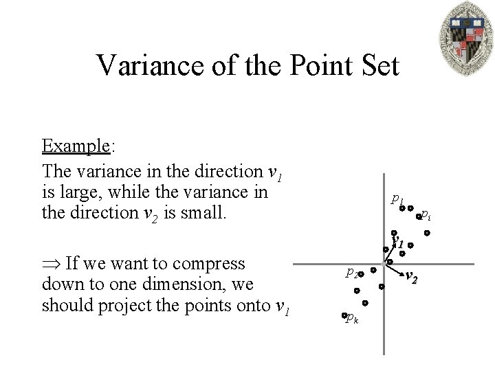
Variance of the Point Set Example: The variance in the direction v 1 is large, while the variance in the direction v 2 is small. If we want to compress down to one dimension, we should project the points onto v 1 pi v 1 p 2 pk v 2

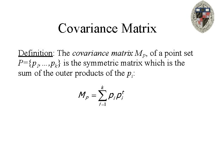
Covariance Matrix Definition: The covariance matrix MP, of a point set P={p 1, …, pk} is the symmetric matrix which is the sum of the outer products of the pi:

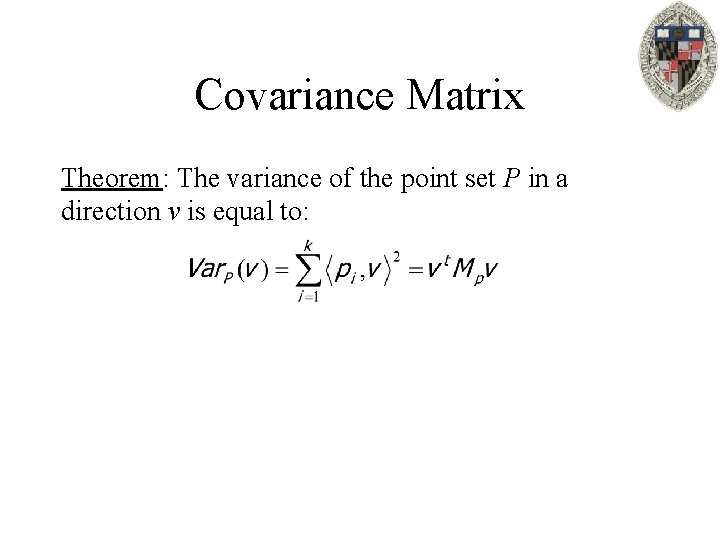
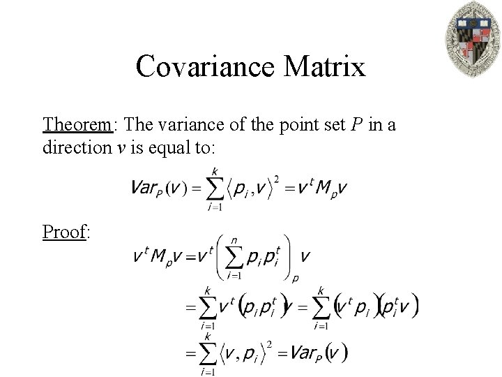
Covariance Matrix Theorem: The variance of the point set P in a direction v is equal to:

Covariance Matrix Theorem: The variance of the point set P in a direction v is equal to: Proof:

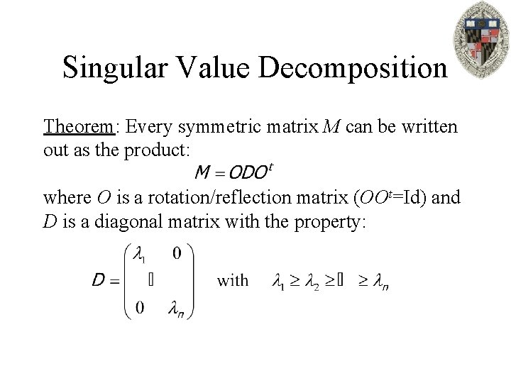
Singular Value Decomposition Theorem: Every symmetric matrix M can be written out as the product: where O is a rotation/reflection matrix (OOt=Id) and D is a diagonal matrix with the property:

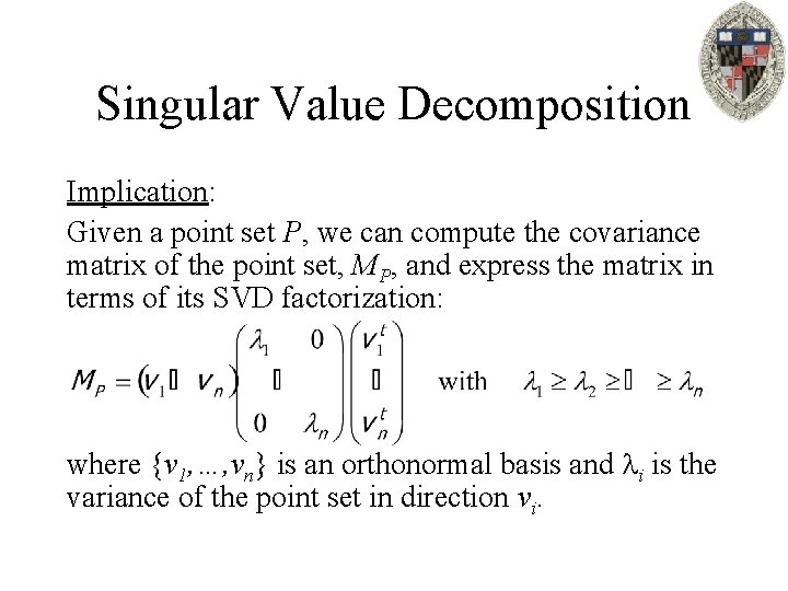
Singular Value Decomposition Implication: Given a point set P, we can compute the covariance matrix of the point set, MP, and express the matrix in terms of its SVD factorization: where {v 1, …, vn} is an orthonormal basis and i is the variance of the point set in direction vi.

Singular Value Decomposition Compression: The vector subspace spanned by {v 1, …, vm} is the vector sub-space that maximizes the variance in the initial point set P. If m is too small, then too much information is discarded and there will be a loss in retrieval accuracy.

Singular Value Decomposition Hierarchical Matching: First coarsely compare the query to database vectors. • If {query is coarsely similar to target} – Refine the comparison • Else – Do not refine O(k n) matching becomes O(k m) with m<<n and no loss of retrieval accuracy.

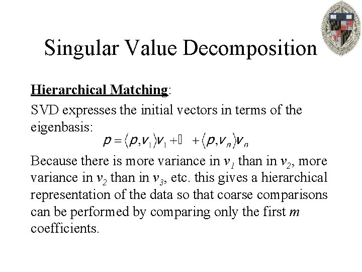
Singular Value Decomposition Hierarchical Matching: SVD expresses the initial vectors in terms of the eigenbasis: Because there is more variance in v 1 than in v 2, more variance in v 2 than in v 3, etc. this gives a hierarchical representation of the data so that coarse comparisons can be performed by comparing only the first m coefficients.

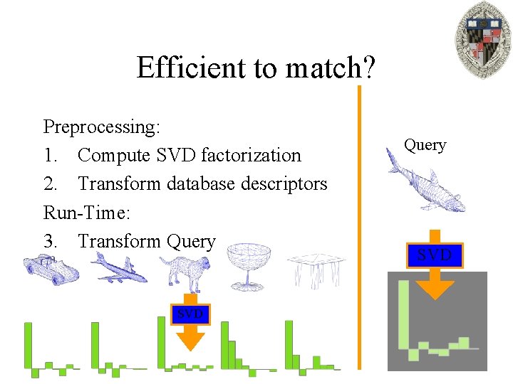
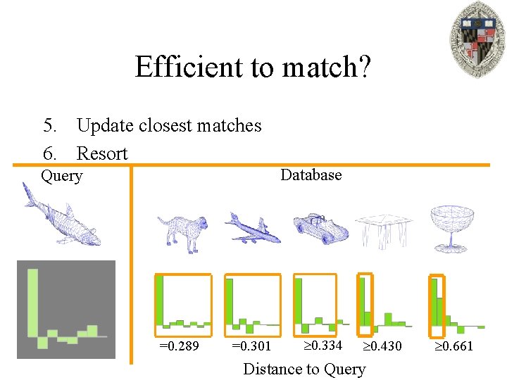
Efficient to match? Preprocessing: 1. Compute SVD factorization 2. Transform database descriptors Run-Time: 3. Transform Query SVD

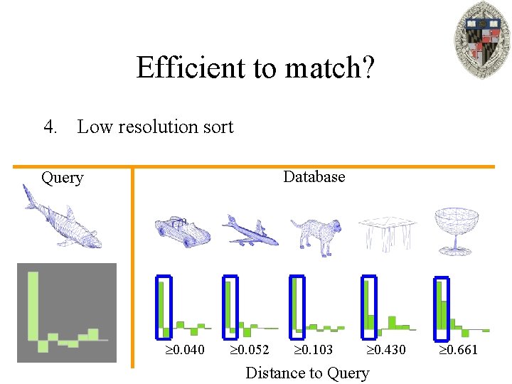
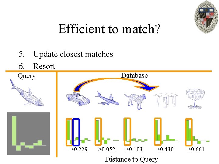
Efficient to match? 4. Low resolution sort Database Query 0. 040 0. 052 0. 103 0. 430 Distance to Query 0. 661

Efficient to match? 5. Update closest matches 6. Resort Database Query 0. 229 0. 052 0. 103 0. 430 Distance to Query 0. 661

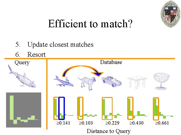
Efficient to match? 5. Update closest matches 6. Resort Database Query 0. 141 0. 103 0. 229 0. 430 Distance to Query 0. 661

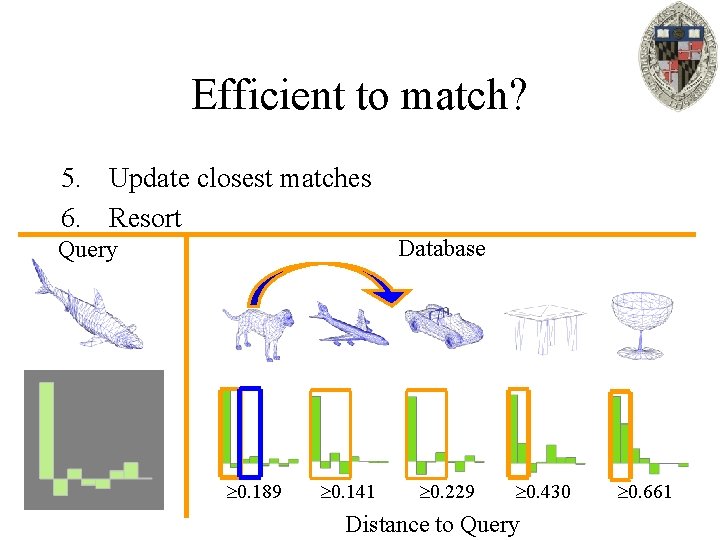
Efficient to match? 5. Update closest matches 6. Resort Database Query 0. 189 0. 141 0. 229 0. 430 Distance to Query 0. 661

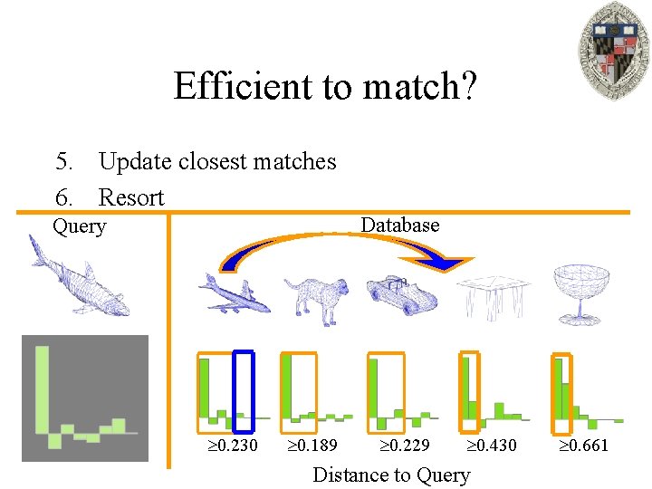
Efficient to match? 5. Update closest matches 6. Resort Database Query 0. 230 0. 189 0. 229 0. 430 Distance to Query 0. 661

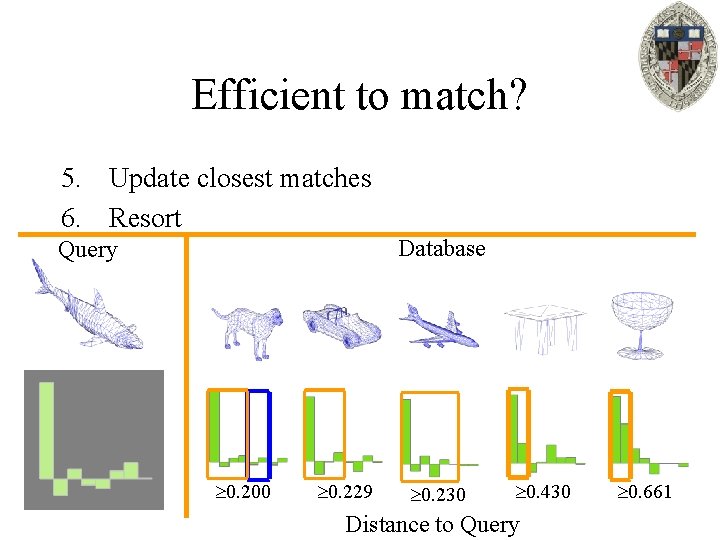
Efficient to match? 5. Update closest matches 6. Resort Database Query 0. 200 0. 229 0. 230 0. 430 Distance to Query 0. 661

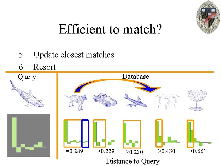
Efficient to match? 5. Update closest matches 6. Resort Database Query =0. 289 0. 229 0. 230 0. 430 Distance to Query 0. 661

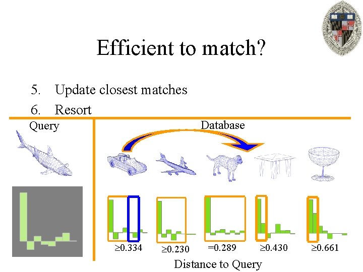
Efficient to match? 5. Update closest matches 6. Resort Database Query 0. 334 0. 230 =0. 289 0. 430 Distance to Query 0. 661

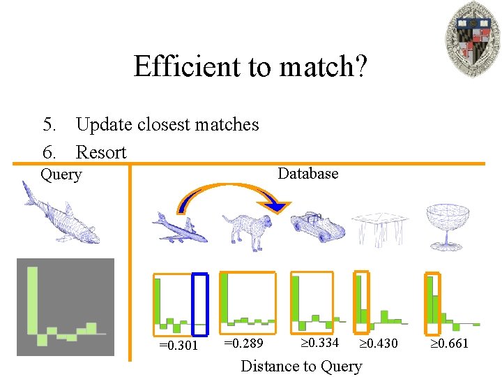
Efficient to match? 5. Update closest matches 6. Resort Database Query =0. 301 =0. 289 0. 334 0. 430 Distance to Query 0. 661

Efficient to match? 5. Update closest matches 6. Resort Database Query =0. 289 =0. 301 0. 334 0. 430 Distance to Query 0. 661

Singular Value Decomposition Theorem: Every symmetric matrix M can be written out as the product: where O is a rotation/reflection matrix (OOt=Id) and D is a diagonal matrix with the property:

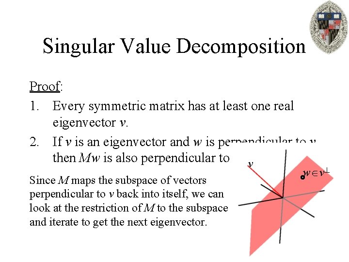
Singular Value Decomposition Proof: 1. Every symmetric matrix has at least one real eigenvector v. 2. If v is an eigenvector and w is perpendicular to v then Mw is also perpendicular to v. v Since M maps the subspace of vectors perpendicular to v back into itself, we can look at the restriction of M to the subspace and iterate to get the next eigenvector. w v

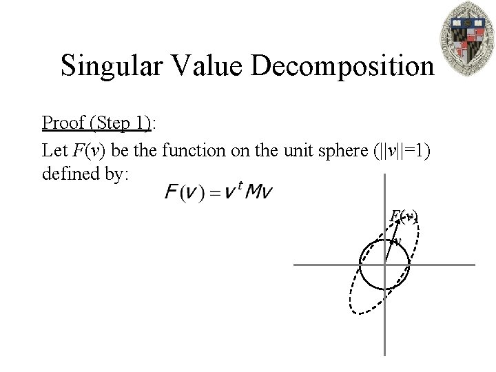
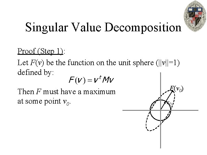
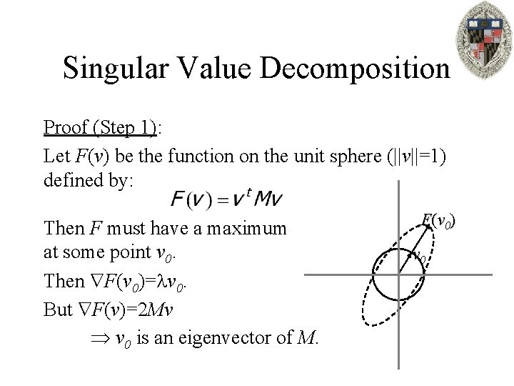
Singular Value Decomposition Proof (Step 1): Let F(v) be the function on the unit sphere (||v||=1) defined by: F (v ) v

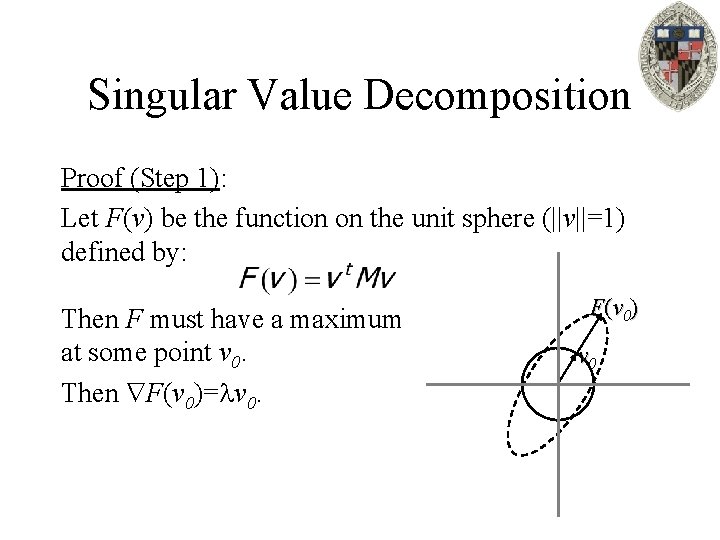
Singular Value Decomposition Proof (Step 1): Let F(v) be the function on the unit sphere (||v||=1) defined by: Then F must have a maximum at some point v 0. F(v 0) v 0

Singular Value Decomposition Proof (Step 1): Let F(v) be the function on the unit sphere (||v||=1) defined by: Then F must have a maximum at some point v 0. Then F(v 0)= v 0. F(v 0) v 0

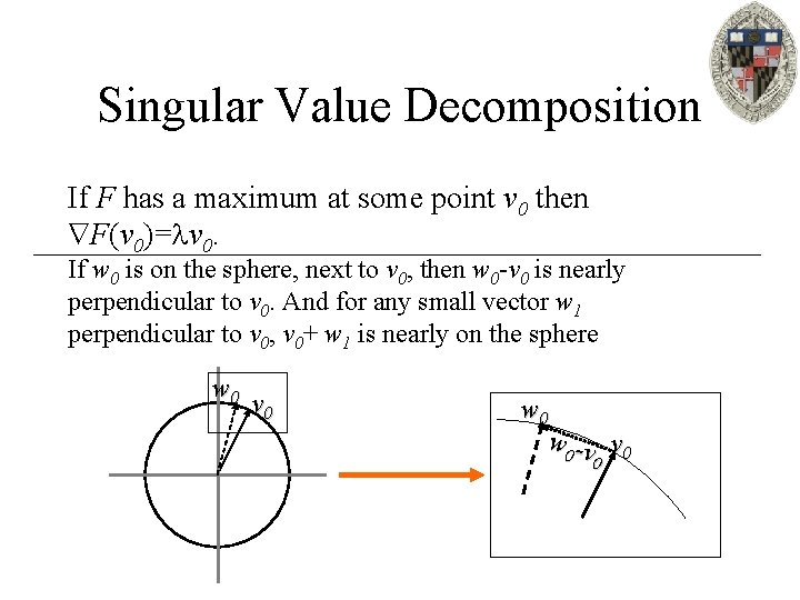
Singular Value Decomposition If F has a maximum at some point v 0 then F(v 0)= v 0. If w 0 is on the sphere, next to v 0, then w 0 -v 0 is nearly perpendicular to v 0. And for any small vector w 1 perpendicular to v 0, v 0+ w 1 is nearly on the sphere w 0 v 0 w 0 -v v 0 0

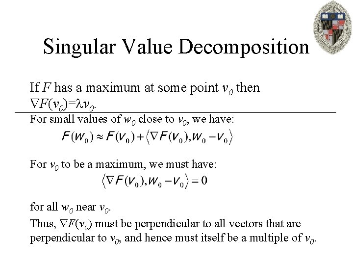
Singular Value Decomposition If F has a maximum at some point v 0 then F(v 0)= v 0. For small values of w 0 close to v 0, we have: For v 0 to be a maximum, we must have: for all w 0 near v 0. Thus, F(v 0) must be perpendicular to all vectors that are perpendicular to v 0, and hence must itself be a multiple of v 0.

Singular Value Decomposition Proof (Step 1): Let F(v) be the function on the unit sphere (||v||=1) defined by: Then F must have a maximum at some point v 0. Then F(v 0)= v 0. F(v 0) v 0

Singular Value Decomposition Proof (Step 1): Let F(v) be the function on the unit sphere (||v||=1) defined by: Then F must have a maximum at some point v 0. Then F(v 0)= v 0. But F(v)=2 Mv v 0 is an eigenvector of M. F(v 0) v 0

Singular Value Decomposition Proof: 1. Every symmetric matrix has at least one eigenvector v. 2. If v is an eigenvector and w is perpendicular to v then Mw is also perpendicular to v.

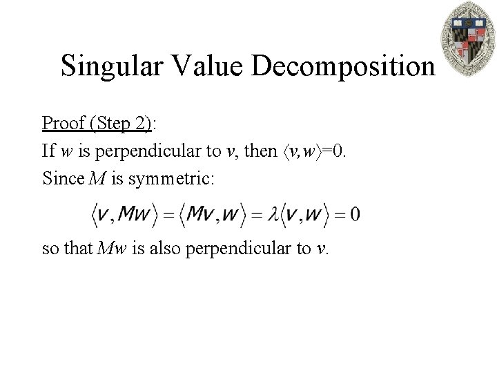
Singular Value Decomposition Proof (Step 2): If w is perpendicular to v, then v, w =0. Since M is symmetric: so that Mw is also perpendicular to v.