Shannons Legacy The Mathematical Parallels Between Packet Switching

Shannon’s Legacy: The Mathematical Parallels Between Packet Switching and Information Transmission Tony T. Lee Department of Information Engineering The Chinese University of Hong Kong December, 2009

Claude Shannon: ‘A mathematical theory of communication’ Bell System Technical Journal 1948

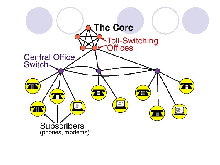
Reliable Communication l Circuit switching network ¡ Reliable communication requires noise-tolerant transmission l Packet switching network ¡ Reliable communication requires both noise-tolerant transmission and contention-tolerant switching

Quantization of Communication Systems l Transmission—from analog channel to digital channel ¡Sampling Theorem of Bandlimited Signal (Whittakev 1915; Nyquist, 1928; Kotelnikou, 1933; Shannon, 1948) l Switching—from circuit switching to packet switching ¡Doubly Stochastic Traffic Matrix Decomposition (Hall 1935; Birkhoff-von Neumann, 1946)

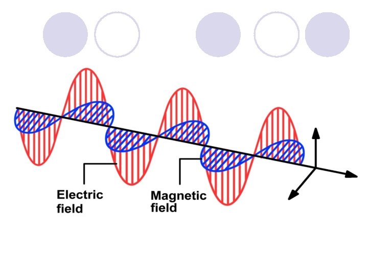
Comparison of Transmission and Switching Shannon’s general communication system Message Source Transmitter Temporal information source: function f(t) of time t Signal Channel capacity C Received signal Receiver Destination Noise source Clos network C(m, n, k) Source Input module nxm o 0 n-1 Central module kxk Output module mxn 0 0 m-1 k-1 Destination o n-1 Spatial information source: function f(i) of space i=0, 1, …, N-1 N-n k-1 N-n N-1 Channel capacity = m Internal contention

Compare Apple with Orange ¡ 350 mg Vitamin C ¡ 500 mg Vitamin C ¡ 1. 5 g/100 g Sugar ¡ 2. 5 g/100 g Sugar

Overview Clos network Communication Channel ¡ Random routing ¡ Noisy channel capacity theorem ¡ Deflection routing ¡ Noisy channel coding theorem ¡ Route assignment ¡ Error-correcting code ¡ Bv. N decomposition ¡ Sampling theorem ¡ Path switching ¡ Noiseless channel ¡ Scheduling ¡ Noiseless coding theorem

Contents l Duality of Noise and Contention l Deflection Routing and Noisy Channel Coding l Route Assignment and Error-Correcting Code l Noiseless Channel Model of Clos Network l Traffic Matrix Decomposition and Sampling theorem l Scheduling and Noiseless Channel Coding

Duality of Transmission and Switching l Transmission channel with noise ¡ Source information is a function of time, errors corrected by providing more signal space ¡ Noise is tamed by error correcting code l Packet switching with contention ¡ Source information f(i) is a function of space, errors corrected by providing more time ¡ Contention is tamed by delay, buffering or deflection Connection request f(i)= j 0111 0001 0101 Message=0101 0100 1101 Delay due to buffering or deflection

Output Contention and Carried Load l Nonblocking switch with uniformly distributed destination address 0 1 • ρ: offered load • ρ’: carried load N-1 l. The difference between offered load and carried load reflects the degree of contention

Proposition on Signal Power of Switch l (V. Benes 63) The energy of connecting network is the number of calls in progress ( carried load ) l The signal power Sp of an N×N crossbar switch is the number of packets carried by outputs, and noise power Np=N- Sp l Pseudo Signal-to-Noise Ratio (PSNR)

Boltzmann Statistics 0 1 2 3 4 5 6 7 a b c d 0 1 2 3 4 5 6 7 n 0 = 5 1 n 1 = 2 0 a n 2 = 1 2 b, c 3 5 4 6 d Micro State Output Ports: Particles Packet: Energy Quantum energy level of outputs = number of packets destined for an output. ni = number of outputs with energy level packets are distinguishable, the total number of states is, N = n 0 + n 1 + L + nr Number of Outputs 7

Boltzmann Statistics (cont’d) l From Boltzmann Entropy Equation • S: Entropy • W: Number of States • C: Boltzman Constant l Maximizing the Entropy by Lagrange Multipliers l Using Stirling’s Approximation for Factorials l Taking the derivatives with respect to ni, yields

Boltzmann Statistics (cont’d) l If offered load on each input is ρ, under uniform loading condition l Probability that there are i packets destined for the output Poisson distribution l Carried load of output

Contention as Pseudo Gaussian Noise l Sum of i. i. d. random variables if output i is busy otherwise Signal power: Noise power: l Sp and Np are Normal rv - Central limit theorem ¡ Signal power Sp is normally distributed ¡ Mean: E[Sp] = Nρ’, Variance: Var[Sp] = Nρ’(1 - ρ’) ¡ Noise power Np is also normally distributed ¡ Mean: E[Np] = N(1 -ρ’), Variance: Var[Np] = Nρ’(1 - ρ’)

Clos Network C(m, n, k) kxk nxm 0 n-1 S n. I n(I+1)-1 0 n-1 0 0 0 G m-1 I n-1 0 G m-1 0 I 0 k-1 0 Q k-1 0 I mxn 0 G m-1 nk-1 0 n-1 k-1 0 I m-1 k-1 Input stage • D = n. Q + R n-1 • D is the destination address D G Q k-1 0 G n-1 0 0 m-1 n(k-1) 0 0 m-1 0 Q k-1 Middle stage 0 G m-1 Q k-1 n. Q 0 n-1 R 0 n. Q+R (n+1)Q-1 n(k-1) n-1 Output stage Slepian-Duguid condition m≥n nk-1 • Q =�D/n�--- output module in the output stage • R = [D] n --- output link in the output module • G is the central module • Routing Tag (G, Q, R)

Connection Matrix 0 1 2 0 0 1 2 3 4 5 1 1 1 3 4 5 6 7 8 2 2 2 6 7 8 Call requests 0 0 0 1 1 1 2 2 2 0 1 2

Clos Network as a Noisy Channel l Source state is a perfect matching l Central modules are randomly assigned to input packets l Offered load on each input link of central module l Carried load on each output link of central module l Pseudo signal-to-noise ratio (PSNR)

Noisy Channel Capacity Theorem l Capacity of the additive white Gaussian noise channel The maximum date rate C that can be sent through a channel subject to Gaussian noise is ¡ C: Channel capacity in bits per second ¡ W: Bandwidth of the channel in hertz ¡ S/N: Signal-to-noise ratio

Tradeoff between Bandwidth and PSNR Circuit switching with nonblocking routing Packet switching with random routing

Clos Network Communication Channel Contention Noise Routing Coding

Contents l Duality of Noise and Contention l Deflection Routing and Noisy Channel Coding l Route Assignment and Error-Correcting Code l Noiseless Channel Model of Clos Network l Traffic Matrix Decomposition and Sampling theorem l Scheduling and Noiseless Channel Coding

Clos Network with Deflection Routing l Route the packets in C(n, n, k) and C(k, k, n) alternately nxn kxk 0 0 k-1 n-1 C(n, n, k) C(k, k, n) Encoding output port addresses in C(n, n, k) Encoding output port addresses in C(k, k, n) Destination: D = n. Q 1 + R 1 Destination: D = k. Q 2 + R 2 Output module number: Output port number: Routing Tag = (Q 1, R 1, Q 2, R 2)

Example of Deflection Routing Deflection 0 1 1 2 5 1 1 0 1 output 1 0 0 1 1 2 0 3 4 1 2 2 1 0 output 2 2 3 0 1 2 1 4 5 2 C(3, 3, 2) C(2, 2, 3) Routing coding in C(3, 3, 2) Routing coding in C(2, 2, 3) Destination Q 1 R 1 Destination Q 2 R 2 0 0 0 1 0 1 2 0 2 2 1 0 3 1 1 4 2 0 5 1 2 5 2 1 1

Analysis of Deflection Clos Network l Markov chain of deflection routing in C(n, n, n) network q q Q R p Input p Probability of success O p Output q=1 -p Probability of deflection

Loss Probability Versus Network Length 0 -2 -4 1 0. 8 -6 0. 4 -8 0. 2 0. 0 0 0. 2 0. 4 0. 6 0. 8 1 0 10 20 30 40 50 60

Loss Probability versus Network Length l The loss probability of deflection Clos network is an exponential function of network length

Shannon’s Noisy Channel Coding Theorem l Given a noisy channel with information capacity C and information transmitted at rate R ¡If R<C, there exists a coding technique which allows the probability of error at the receiver to be made arbitrarily small. ¡If R>C, the probability of error at the receiver increases without bound.

Binary Symmetric Channel l The Binary Symmetric Channel(BSC) with cross probability q=1 -p‹½ has capacity 0 q p 0 p 1 q 1 l There exist encoding E and decoding D functions l If the rate R=k/n=C-δ for some δ>0. The error probability is bounded by l If R=k/n=C+ δ for some δ>0, the error probability is unbounded

Parallels Between Noise and Contention Binary Symmetric Channel Deflection Clos Network Cross Probability q<½ Deflection Probability q<½ Random Coding Deflection Routing R≤C R≤n Exponential Error Probability Exponential Loss Probability Complexity Increases with Code Length n Complexity Increases with Network Length L Typical Set Decoding Equivalent Set of Outputs

Contents l Duality of Noise and Contention l Deflection Routing and Noisy Channel Coding l Route Assignment and Error-Correcting Code l Noiseless Channel Model of Clos Network l Traffic Matrix Decomposition and Sampling theorem l Scheduling and Noiseless Channel Coding

Hall’s Marriage Theorem Let G be a bipartite graph with input set VI, and edge set E. There exists a perfect matching f: VI → VO, if and only if for every subset A ⊂ VI, |NA| ≥ |A| where NA is the neighborhood of set A, NA = {b | (a, b) ∈ E, a∈A} ⊆ VO A A For subset A, |A|=2 |NA| = 4

Edge Coloring of Bipartite Graph l A Regular bipartite graph G with vertex-degree m satisfies Hall’s condition l Let A ⊆ VI be a set of inputs, NA = {b | (a, b) ∈ E, a∈A} , since edges terminate on vertices in A must be terminated on NA at the other end. Then m|NA| ≥ m|A|, so |N A| ≥ |A|

Route Assignment in Clos Network 0 1 0 0 2 3 2 1 3 3 4 2 6 7 1 1 4 5 1 2 5 6 2 3 7 Computation of routing tag (G, Q, R) S=Input 0 1 2 3 4 5 6 7 D=Output 1 3 2 0 6 4 7 5 G=Central module 0 2 2 1 0 2 0 1 1 0 3 2 1 1 0 0 1 1

Rearrangeabe Clos Network and Channel Coding Theorem l (Slepian-Duguid) Every Clos network with m≥n is rearrangeably nonblocking ¡ The bipartite graph with degree n can be edge colored by m colors if m≥n ¡ There is a route assignment for any permutation l Shannon’s noisy channel coding theorem ¡ It is possible to transmit information without error up to a limit C.

Gallager Codes l Low Density Parity Checking (Gallager 60) l Bipartite Graph Representation (Tanner 81) l Approaching Shannon Limit (Richardson 99) VL: n variables 0 x 0 1 x 1 0 x 2 0 x 3 1 x 4 1 x 5 0 x 6 1 x 7 VR: m constraints x 1+x 3+x 4+x 7=1 + + Unsatisfied x 0+x 1+x 2+x 5=0 Satisfied x 2+x 5+x 6+x 7=0 Satisfied x 0+x 3+x 4+x 6=1 Unsatisfied Closed Under (+)2

Expander Codes l Expander Graph G(VL, VR, E) ¡ VL: k-regular with |VL| = n ¡ VR: 2 k-regular with |VR|=n/2 ¡ There exists α>0, such that for every S ⊂ VL |S| < αn |NS| > (k/2)|S| l Distance(C(G))> αn l Decoding Algorithm (Sipser-Speilman 95) If there is a vertex v∈ VL such that most of its neighbors (checks) are unsatisfied, flip the value of v. Repeat l The Algorithm can remove up to (αn)/2 errors If for every S ⊂ VL

Benes Network Bipartite graph of call requests 1 2 0 3 4 5 6 x 1 G(VL X VR, E) 1 2 3 4 5 6 1 7 8 + x 1 + x 2 =1 x 2 + x 3 + x 4 =1 Input Module x 3 + x 5 + x 6 =1 Constraints x 4 + x 7 + x 8 =1 x 5 + x 1 + x 3 =1 x 6 + x 8 =1 x 7 + x 4 + x 7 =1 x 8 + x 2 + x 5 =1 7 8 Not closed under + Output Module Constraints

Bipartite Matching and Route Assignments Call requests 1 2 3 4 5 6 7 8 1 1 2 2 3 3 4 4 Bipartite Matching and Edge Coloring

Flip Algorithm l Assign x 1=0, x 2=1, x 3=0, x 4=1…to satisfy all input module constraints initially l Unsatisfied vertices divide each cycle into segments. Label them α and β alternately and flip values of all variables in α segments x 1+x 2=1 + x 2 x 3+x 4=1 + x 4 x 5+x 6=1 x 7+x 8=1 + + x 6 x 7 x 8 Input module constraints 0 1 0 + x 1+x 3=0 + x 6+x 8=0 + x 4+x 7=1 1 0 1 variables + x 2+x 5=1 Output module constraints

Final Route Assignments Apply the algorithm iteratively to complete the route assignments 1 1 2 2 3 3 4 4 5 5 6 6 7 7 8 8

Contents l Duality of Noise and Contention l Deflection Routing and Noisy Channel Coding l Route Assignment and Error-Correcting Code l Noiseless Channel Model of Clos Network l Traffic Matrix Decomposition and Sampling theorem l Scheduling and Noiseless Channel Coding

Concept of Path Switching l Traffic signal at cross-roads N Traffic loading: NS: 2ρ EW: ρ W E S NS traffic EW traffic Cycle l Use predetermined conflict-free states in cyclic manner l The duration of each state in a cycle is determined by traffic loading l Distributed control

Path Switching of Clos Network 0 0 1 2 3 4 5 1 1 1 3 4 5 6 7 8 2 2 2 6 7 8 1 2 0 0 0 1 1 2 2 Time slot 1 1 Time slot 2 2

Capacity of Virtual Path l Capacity equals average number of edges Time slot 0 Virtual path 0 0 1 1 2 2 G 1 Time slot 1 G 1 U G 2 0 0 1 1 2 2 G 2

Noiseless Virtual Path of Clos Network Input module (input queued switch) o n-1 nxm kxk 0 0 0 k-1 m-1 k-1 Buffer and scheduler Scheduling to combat channel noise Input module i Virtual path Output module (output queued Switch) o n-1 Predetermined connection pattern in every time slot Input buffer λij Source Central module (nonblocking switch) mxn Output buffer Input module j Buffer Destination and scheduler Buffering to combat source noise

Contents l Duality of Noise and Contention l Deflection Routing and Noisy Channel Coding l Route Assignment and Error-Correcting Code l Noiseless Channel Model of Clos Network l Traffic Matrix Decomposition and Sampling theorem l Scheduling and Noiseless Channel Coding

Complexity Reduction of Permutation Space Subspace spanned by K base states {Pi} Convex hull of doubly stochastic matrix l Reduce the complexity of permutation space from N! to K • K ≤ min{F, N 2 -2 N+2}, the base dimension of C • K ≤ F ≤(BN)/m, if C is bandlimited cij ≤B/F • K ≤ F can be a constant independent of N if round-off error of order 1/F is acceptable

Parallels Between Sampling Theorems Network environment Packet switching Digital transmission Time slotted switching system Time slotted transmission system Capacity limited traffic matrix Bandwidth limited signal function Complete matching, (0, 1) Permutation matrixes Entropy, (0, 1) Binary sequences Birkhoff decomposition (Hall’s matching theorem) Fourier series Bandwidth limitation Samples Expansion

Parallels Between Sampling Theorems Inversion by weighted sum by samples Complexity reduction Qo. S Packet switching Digital transmission Reconstruction the capacity by running sum Reconstruction the signal by interpolation l. Reduce number of permutation from N! to O(N 2). l Reduce to O(N), if bandwidth is Reduce infinite dimensional signal limited. space to finite number 2 t. W in any l. Reduce to constant F if truncation duration t. error of order O( 1 / F ) is acceptable. Buffering and scheduling, capacity guarantee, delay bound Pulse code modulation (PCM), error-correcting code, data compression, DSP

Contents l Duality of Noise and Contention l Deflection Routing and Noisy Channel Coding l Route Assignment and Error-Correcting Code l Noiseless Channel Model of Clos Network l Traffic Matrix Decomposition and Sampling theorem l Scheduling and Noiseless Channel Coding

Source Coding and Scheduling l Source coding: A mapping from code book to source symbols to reduce redundancy l Scheduling: A mapping from predetermined connection patterns to incoming packets to reduce delay jitter

Smoothness of Scheduling l Scheduling of a set of permutation matrices generated by decomposition with frame size F Pi Pi Pi F l The sequence , , ……, of inter-state distance of state P i within a period of F satisfies l Smoothness of state Pi

Entropy of Decomposition and Smoothness of Scheduling l Any scheduling of capacity decomposition (Kraft’s Inequality) l Entropy inequality The equality holds when

Smoothness of Scheduling l A Special Case ¡ If K=F, Фi=1/F, and ni=1 for all i, then for all i=1, …, F Smoothness l Another Example The Input Set The Expected Optimal Result P 1 P 2 P 1 P 3 P 1 P 2 P 1 P 4

Smoothness of optimal scheduling l Smoothness of random scheduling l Kullback-Leibler distance reaches maximum when l Always possible to device a scheduling within 1/2 of entropy

Noiseless Coding Theorem l Necessary and Sufficient condition to prefix encode values x 1, x 2, …, x. N of X with respective length n 1, n 2, …n. N (Kraft’s Inequality) l Any prefix code that assigns ni bits to xi l Always possible to device a prefix code within 1 of entropy

Weighted Fair Queueing (WFQ) Scheduling Algorithm l The WFQ Scheduling Algorithm Select the state with the smallest finish time and increase its finish time by the inverse of its weight. Repeat this process until the frame size is reached P 1 P 2 P 3 P 4 P 5 Selection 1 2 8 8 P 1 2 4 8 8 P 1 3 6 8 8 P 1 4 8 8 8 P 1 5 10 8 8 P 2 6 10 16 8 8 8 P 3 7 10 16 16 8 8 P 4 8 10 16 16 16 8 P 5 The Final Sequence Should be P 1 P 1 P 2 P 3 P 4 P 5

WF 2 Q Scheduling Algorithm WF 2 Q incorporates rate requirement of generalized processor sharing (GPS) in the WFQ. Let Ti(τ) be the number of time slots assigned to state Pi up to time τ, the WF 2 Q will select the state Pi that satisfies in every time slot τ = 1, 2, . . . Same example P 1 P 2 P 3 P 4 P 5 1 2 8 8 P 1 P 2 P 3 P 4 P 5 P 1 2 4 8 8 P 2 P 3 P 4 P 5 P 2 3 4 8 8 P 1 P 3 P 4 P 5 P 1 4 4 16 8 8 8 P 3 P 4 P 5 P 3 5 6 16 8 8 8 P 1 P 4 P 5 P 1 6 6 16 16 8 8 P 4 P 5 P 4 7 8 16 16 8 8 P 1 P 5 P 1 8 10 16 16 16 8 P 5 The Final Sequence P 1 P 2 P 1 P 3 P 1 P 4 P 1 P 5 Selection

Huffman Round Robin (Hu. RR) Algorithm Step 1 Initially set the root be temporary node Px, and S = Px…Px be temporary sequence. Step 2 Apply the WFQ to the two successors of Px to produce a sequecne T, and substitute T for the subsequence Px…Px of S. Step 3 If there is no intermediate node in the sequence S, then terminate the algorithm. Otherwise select an intermediate node Px appearing in S and go to step 2. 1 PZ PX P 1 0. 5 P 2 0. 125 0. 5 PY 0. 25 P 3 0. 125 P 4 0. 125 0. 25 P 5 0. 125 Huffman Code logarithm of interstate time = length of Huffman code

Comparison of Scheduling Algorithms P 1 P 2 P 3 P 4 Random WFQ WF 2 Q Hu. RR Entropy 0. 1 0. 7 1. 628 1. 575 1. 414 1. 357 0. 1 0. 2 0. 6 1. 894 1. 734 1. 626 1. 604 1. 571 0. 3 0. 5 2. 040 1. 784 1. 724 1. 702 1. 686 0. 1 0. 2 0. 5 2. 123 1. 882 1. 801 1. 772 1. 761 0. 4 2. 086 1. 787 1. 745 1. 722 0. 1 0. 2 0. 3 0. 4 2. 229 1. 903 1. 884 1. 847 0. 2 0. 4 2. 312 2. 011 1. 980 1. 933 1. 922 0. 1 0. 3 2. 286 1. 908 1. 896 0. 2 0. 3 2. 370 2. 016 1. 980 1. 971 Better Performance

Entropy of Capacity Matrix C=[cij] l Entropy of input module i is l Input entropies: l Entropy of output module j is l Output entropies: l Entropy of capacity matrix C:

Entropy of Capacity Matrix (Cont’d) l Given capacity matrix C = [cij] l Input entropy H and output entropy H are l Entropy of capacity matrix C is

Two-Dimensional Smoothness l Inter-token times satisfies where nij is the number of tokens assigned to virtual path V ij within a frame F l Smoothness of virtual path Vij

Two-Dimensional Smoothness (Cont’d) l Smoothness of input module i l Input smoothness: l Smoothness of output module j l Output smoothness: l 2 D-Smoothness of scheduling

Theorem: For any 2 D-scheduling of the capacity matrix decomposition , we have 1. Kraft’s matrix Kr =[2 -dij] is doubly sub-stochastic 2. for input module i=1, 2, …, N 3. for output module j = 1, 2, …, N 4. The above equalities hold when and k = 1, 2, …, nij. , for i, j = 1, 2, …, N

2 D-Smoothness of WFQ l Decomposition of matrix C with frame size 8 P 1 P 2 P 3 P 4 P 5 l WFQ scheduling W F Q Input Smoothness Output Smoothness a, b, c, d are tokens assigned to input 1 -4

2 D-Smoothness of Hu. RR l Hu. RR scheduling algorithm H u R R l Improved smoothness with Hu. RR

Improving 2 D-Smoothness l Decomposition with less matrices P 1 P 2 P 3 P 4 l Hu. RR scheduling H u R R Input Smoothness Improvement for input 3 Output Smoothness Improvement for output 4

Transmission-Switching Dual of Communication Permutation Matrix Clos Network Route Assignment Hall’s Matching Scheduling Theorem and Buffering (Bv. N Decomposition) Boltzmann Equation S = k log. W Communication System Entropy Noisy Channel Coding Bandlimited Sampling Theorem Source Coding

Conclusion-it is law of probability l Input signal to transmission system is a function of time l The main theorem on noisy channel coding is proved by law of large number l Input signal to switching system is a function of space l Both theorems on deflection routing and smoothness of scheduling are proved by randomness

Conclusion-it is law of probability l Input signal to transmission system is a function of time l The main theorem on noisy channel coding is proved by law of large number l Input signal to switching system is a function of space l Both theorems on deflection routing and smoothness of scheduling are proved by randomness

Transmission-Switching Dual of Communication Permutation Matrix Clos Network Route Assignment Hall’s Matching Scheduling Theorem and Buffering (Bv. N Decomposition) Boltzmann Equation S = k log. W Communication System Entropy Noisy Channel Coding Bandlimited Sampling Theorem Source Coding

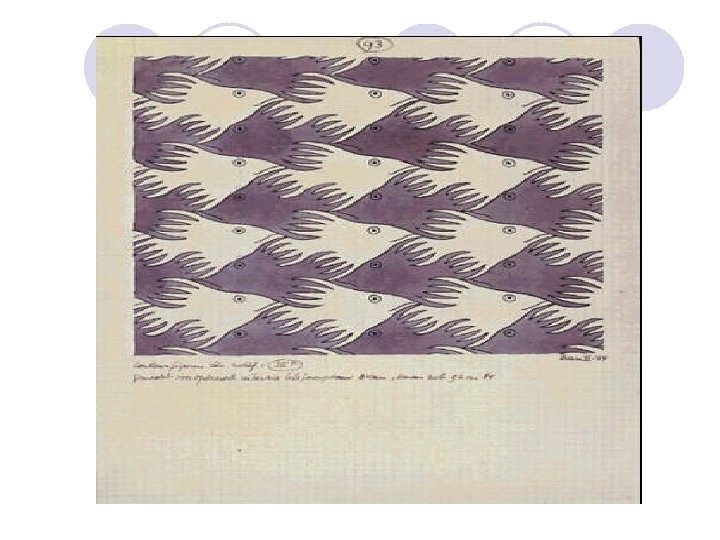
The universe is built on a plan of profound symmetry of which is somehow present in the inner structure of our intellect. -Paul Valery (1871 -1945)