Session VISION GRAPHICS AND ROBOTICS Map Building without

Session : VISION, GRAPHICS AND ROBOTICS Map Building without Localization by Dimensionality Reduction Techniques Takehisa YAIRI RCAST, University of Tokyo
Outline • Background – Motivation, Purpose and Problem to consider • Related Works – SLAM, and Mapping with DR methods • Proposed Framework - LFMDR – Basic idea, Assumptions, Formalization • Experiment – Visibility-Only and Bearing-Only Mappings • Conclusion

Motivation • Map building – An essential capability for intelligent agents • SLAM (Simultaneous Localization and Mapping) – Has been mainstream for many years – Very successful both in theory and practice • I like SLAM too, but I feel something’s missing. . – Are the mapping and localization really inseparable ? – Are the motion and measurement models necessary ? – How about the aspect of map building as an abstraction of the world ? • Is there another map building framework ?
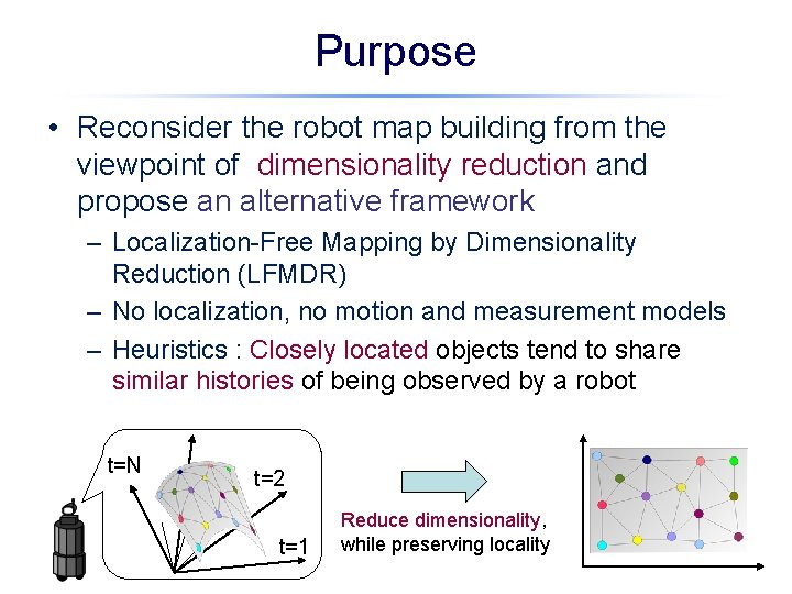
Purpose • Reconsider the robot map building from the viewpoint of dimensionality reduction and propose an alternative framework – Localization-Free Mapping by Dimensionality Reduction (LFMDR) – No localization, no motion and measurement models – Heuristics : Closely located objects tend to share similar histories of being observed by a robot t=N t=2 t=1 Reduce dimensionality, while preserving locality

Map Building Problem to Consider • Feature-based map (i. e. Not topological, not occupancy-grid) – A map is represented by 2 -D coordinates of objects • There EXIST motion and measurement models – But, they are not necessarily known in advance Positions of objects Observation State Move m Motion model (State transition model) Measurement model (Observation model) Exist, but may be unknown
![Related Works : SLAM [Thrun 02] • Problem : “Estimate m and x 1: Related Works : SLAM [Thrun 02] • Problem : “Estimate m and x 1:](http://slidetodoc.com/presentation_image_h2/b6b145e618ae66907518b0027dc83b7f/image-6.jpg)
Related Works : SLAM [Thrun 02] • Problem : “Estimate m and x 1: t from y 1: t , given f and g” • Solutions: – Kalman Filter with extended state – Incremental maximum likelihood [Thrun, et. al. 98] – Rao-Blackwellized Particle Filter [Montemerlo, et. al. 02] • Motion and measurement models must be given • Estimations of map and robot position are coupled Given: Motion model Measurement model Input: Measurement data Output: Map Robot trajectory
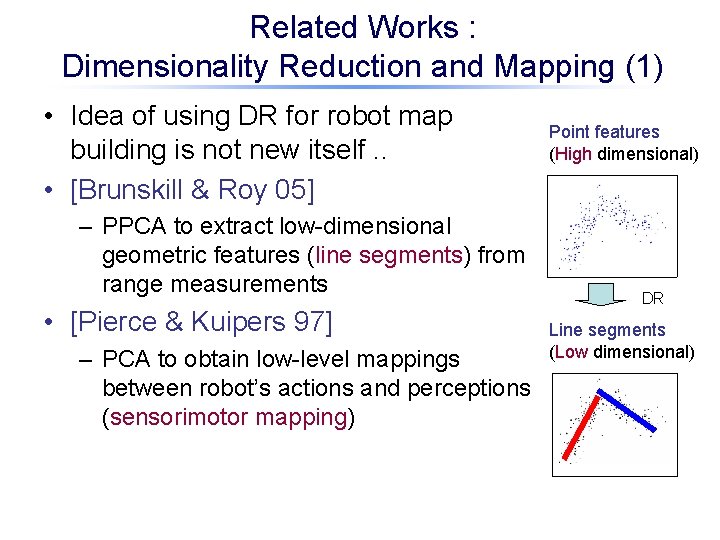
Related Works : Dimensionality Reduction and Mapping (1) • Idea of using DR for robot map building is not new itself. . • [Brunskill & Roy 05] – PPCA to extract low-dimensional geometric features (line segments) from range measurements • [Pierce & Kuipers 97] – PCA to obtain low-level mappings between robot’s actions and perceptions (sensorimotor mapping) Point features (High dimensional) DR Line segments (Low dimensional)
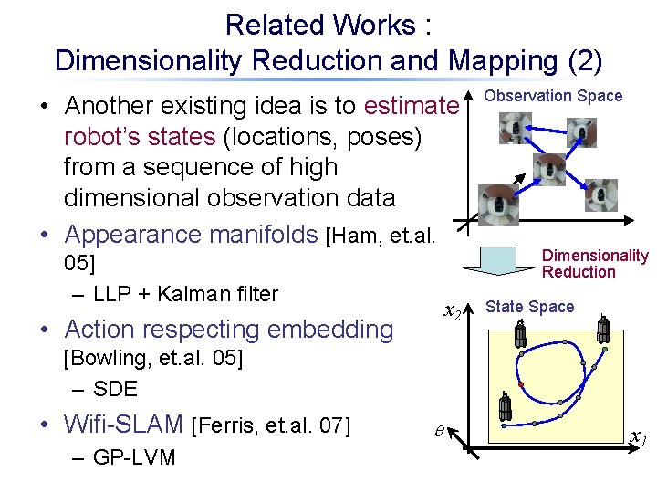
Related Works : Dimensionality Reduction and Mapping (2) • Another existing idea is to estimate robot’s states (locations, poses) from a sequence of high dimensional observation data • Appearance manifolds [Ham, et. al. 05] – LLP + Kalman filter x 2 • Action respecting embedding Observation Space Dimensionality Reduction State Space [Bowling, et. al. 05] – SDE • Wifi-SLAM [Ferris, et. al. 07] – GP-LVM q x 1
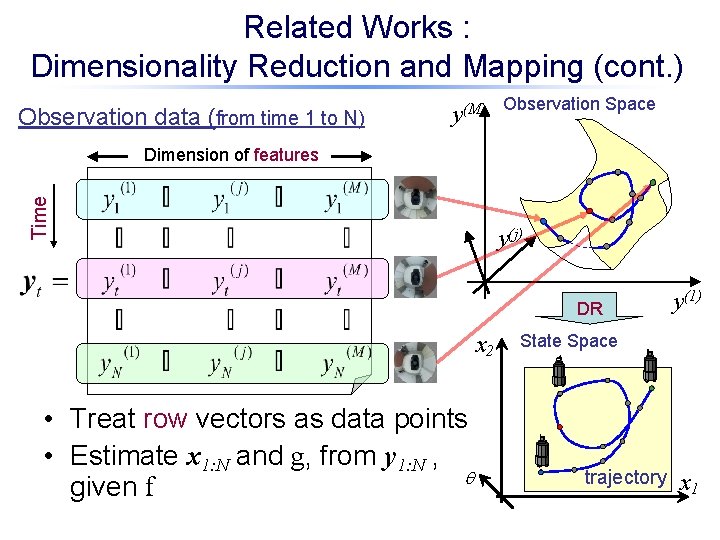
Related Works : Dimensionality Reduction and Mapping (cont. ) Observation data (from time 1 to N) y(M) Observation Space Time Dimension of features y(j) DR x 2 • Treat row vectors as data points • Estimate x 1: N and g, from y 1: N , q given f y(1) State Space trajectory x 1
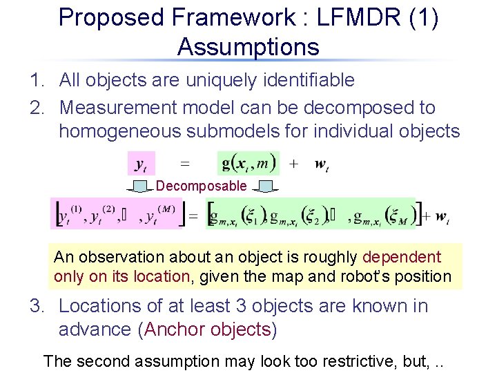
Proposed Framework : LFMDR (1) Assumptions 1. All objects are uniquely identifiable 2. Measurement model can be decomposed to homogeneous submodels for individual objects Decomposable An observation about an object is roughly dependent only on its location, given the map and robot’s position 3. Locations of at least 3 objects are known in advance (Anchor objects) The second assumption may look too restrictive, but, . .
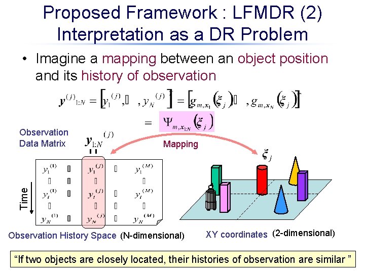
Proposed Framework : LFMDR (2) Interpretation as a DR Problem • Imagine a mapping between an object position and its history of observation Mapping Time Observation Data Matrix Observation History Space (N-dimensional) XY coordinates (2 -dimensional) “If two objects are closely located, their histories of observation are similar ”
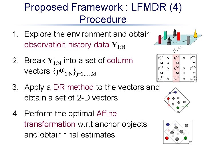
Proposed Framework : LFMDR (4) Procedure 1. Explore the environment and obtain observation history data Y 1: N 2. Break Y 1: N into a set of column vectors {y(j)1: N}j=1, …, M 3. Apply a DR method to the vectors and obtain a set of 2 -D vectors 4. Perform the optimal Affine transformation w. r. t anchor objects, and obtain final estimates
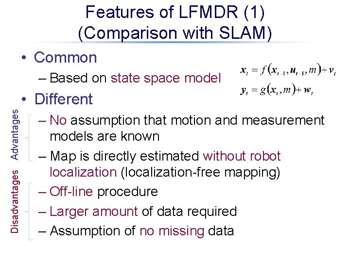
Features of LFMDR (1) (Comparison with SLAM) • Common – Based on state space model Disadvantages Advantages • Different – No assumption that motion and measurement models are known – Map is directly estimated without robot localization (localization-free mapping) – Off-line procedure – Larger amount of data required – Assumption of no missing data
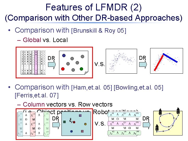
Features of LFMDR (2) (Comparison with Other DR-based Approaches) • Comparison with [Brunskill & Roy 05] – Global vs. Local DR v. s. DR • Comparison with [Ham, et. al. 05] [Bowling, et. al. 05] [Ferris, et. al. 07] – Column vectors vs. Row vectors (i. e. , Object positions vs. Robot positions) DR v. s. DR
![Experiment • Applied to 2 different situations – [Case 1] Visibility-only mapping – [Case Experiment • Applied to 2 different situations – [Case 1] Visibility-only mapping – [Case](http://slidetodoc.com/presentation_image_h2/b6b145e618ae66907518b0027dc83b7f/image-15.jpg)
Experiment • Applied to 2 different situations – [Case 1] Visibility-only mapping – [Case 2] Bearing-only mapping • Common settings: – 2. 5[m]x 2. 5[m] square region – 50 objects (incl. 4 anchors) – Exploration with random direction change and obstacle avoidance WEBOTS simulator • Evaluation – Mean Position Error (MPE) – Mean Orientation Error (MOE) – Averaged over 25 runs Triangle Orientation A C A-B-C Difference B B A A-C-B C
![DR Methods 1. Linear PCA 2. SMACOF-MDS [De. Leeuw 77] (a) Equal weights, (b) DR Methods 1. Linear PCA 2. SMACOF-MDS [De. Leeuw 77] (a) Equal weights, (b)](http://slidetodoc.com/presentation_image_h2/b6b145e618ae66907518b0027dc83b7f/image-16.jpg)
DR Methods 1. Linear PCA 2. SMACOF-MDS [De. Leeuw 77] (a) Equal weights, (b) k. NN-based weighting 3. Kernel PCA [Scholkopf, et. al. 98] (a) Gaussian, (b) Polynomial 4. ISOMAP [Tennenbaum, et. al. 00] 5. LLE [Roweis&Saul 00] 6. Laplacian Eigenmap [Belkin&Niyogi 02] 7. Hessian LLE [Donoho&Grimes 03] 8. SDE [Weinberger, et. al. 05] Parameters (k, s 2, d) were tuned manually
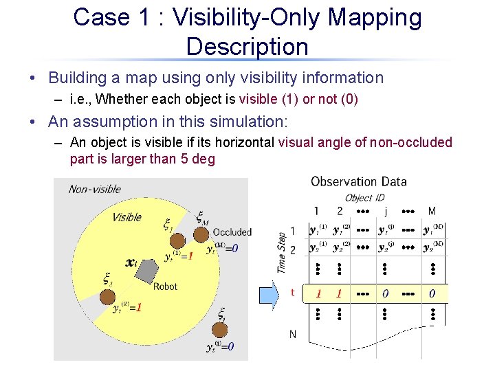
Case 1 : Visibility-Only Mapping Description • Building a map using only visibility information – i. e. , Whether each object is visible (1) or not (0) • An assumption in this simulation: – An object is visible if its horizontal visual angle of non-occluded part is larger than 5 deg
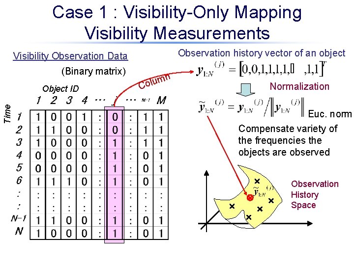
Case 1 : Visibility-Only Mapping Visibility Measurements Observation history vector of an object Visibility Observation Data (Binary matrix) Time Object ID n m Colu Normalization Euc. norm Compensate variety of the frequencies the objects are observed Observation History Space
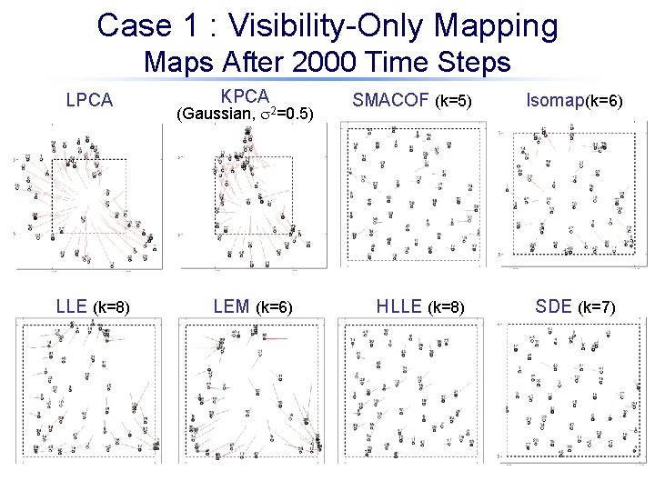
Case 1 : Visibility-Only Mapping Maps After 2000 Time Steps LPCA LLE (k=8) KPCA (Gaussian, s 2=0. 5) LEM (k=6) SMACOF (k=5) HLLE (k=8) Isomap(k=6) SDE (k=7)
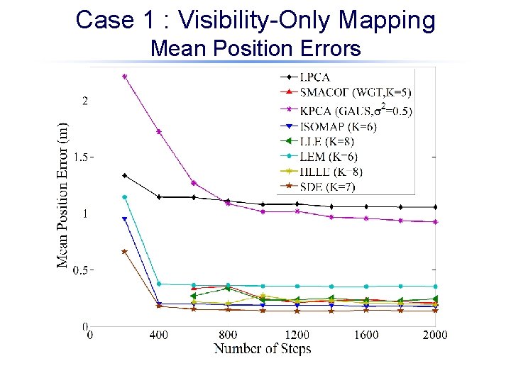
Case 1 : Visibility-Only Mapping Mean Position Errors
![Case 1 : Visibility-Only Mapping Final Map Errors DR methods Opt. param. MPE [m] Case 1 : Visibility-Only Mapping Final Map Errors DR methods Opt. param. MPE [m]](http://slidetodoc.com/presentation_image_h2/b6b145e618ae66907518b0027dc83b7f/image-21.jpg)
Case 1 : Visibility-Only Mapping Final Map Errors DR methods Opt. param. MPE [m] Rnk LPCA(CMDS) SMA(UNWGT) SMA(WGT) KPCA(GAUS) KPCA(POLY) ISOMAP LLE LEM HLLE SDE K=5 s 2 = 0. 5 d=8 K=6 K=8 K=7 1. 055 10 0. 421 7 0. 206 4 0. 926 8 0. 953 9 0. 177 2 0. 241 5 0. 352 6 0. 192 3 0. 138 1 MOE[%] Rnk 18. 19 8 5. 86 6 4. 83 4 23. 29 9 27. 03 10 4. 11 2 5. 4 5 8. 17 7 4. 24 3 3. 65 1
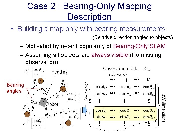
Case 2 : Bearing-Only Mapping Description • Building a map only with bearing measurements (Relative direction angles to objects) – Motivated by recent popularity of Bearing-Only SLAM – Assuming all objects are always visible (No missing observation) Bearing angles
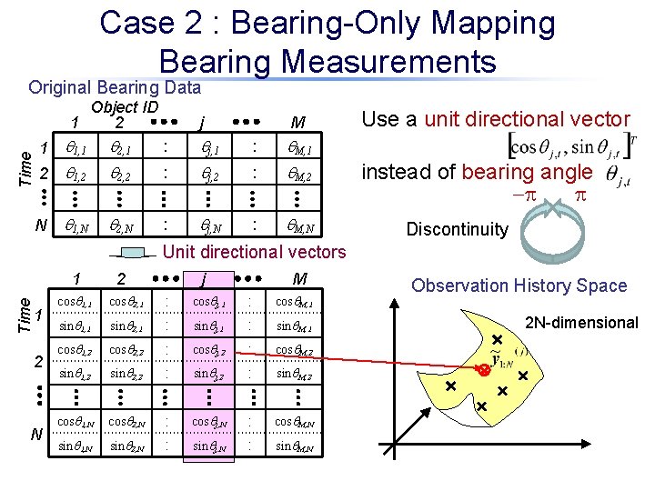
Case 2 : Bearing-Only Mapping Bearing Measurements Original Bearing Data Time Object ID 1 2 j M 1 q 1, 1 q 2, 1 : qj, 1 : q. M, 1 2 q 1, 2 q 2, 2 : qj, 2 : q. M, 2 N q 1, N q 2, N : qj, N : q. M, N Use a unit directional vector instead of bearing angle -p p Discontinuity Unit directional vectors Time 1 1 2 N 2 j M cosq 1, 1 cosq 2, 1 : cosqj, 1 : cosq. M, 1 sinq 1, 1 sinq 2, 1 : sinqj, 1 : sinq. M, 1 cosq 1, 2 cosq 2, 2 : cosqj, 2 : cosq. M, 2 sinq 1, 2 sinq 2, 2 : sinqj, 2 : sinq. M, 2 cosq 1, N cosq 2, N : cosqj, N : cosq. M, N sinq 1, N sinq 2, N : sinqj, N : sinq. M, N Observation History Space 2 N-dimensional
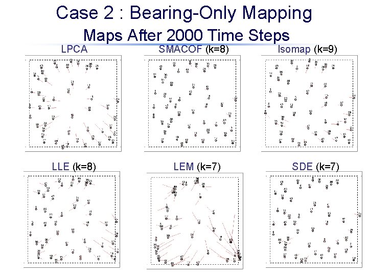
Case 2 : Bearing-Only Mapping Maps After 2000 Time Steps LPCA LLE (k=8) SMACOF (k=8) LEM (k=7) Isomap (k=9) SDE (k=7)
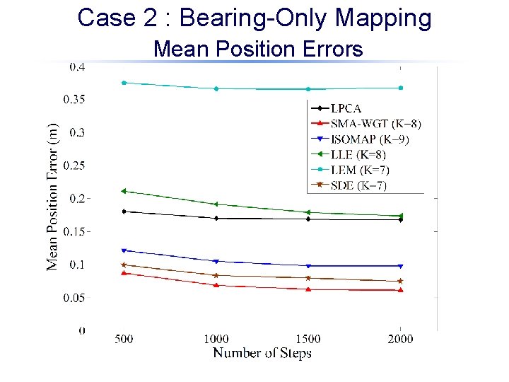
Case 2 : Bearing-Only Mapping Mean Position Errors
![Case 2 : Bearing-Only Mapping Final Map Errors DR methods Opt. param. MPE [m] Case 2 : Bearing-Only Mapping Final Map Errors DR methods Opt. param. MPE [m]](http://slidetodoc.com/presentation_image_h2/b6b145e618ae66907518b0027dc83b7f/image-26.jpg)
Case 2 : Bearing-Only Mapping Final Map Errors DR methods Opt. param. MPE [m] Rnk LPCA(CMDS) SMA(UNWGT) SMA(WGT) KPCA(GAUS) KPCA(POLY) ISOMAP LLE LEM HLLE SDE K=8 s 2=1. 0 d=2 K=9 K=8 K=7 0. 168 0. 101 0. 0609 3. 47 0. 605 0. 0979 0. 173 0. 367 NA 0. 0741 5 4 1 9 8 3 6 7 2 MOE[%] Rnk 2. 33 5 1. 38 3 1 1 49. 2 9 9. 15 8 1. 83 4 3. 03 6 8. 46 7 NA 1. 36 2 (*) It might imply the distribution approaches to linear
Conclusion • Reconsidered robot map building from the viewpoint of dimensionality reduction • Proposed a new framework named LFMDR – Motion and measurement models are not required – Not need to estimate robot’s poses (localization-free) – However, larger amount of data is needed • Tested on two types of sensor measurements – Visibility information, and Bearing angles • Compared a variety of DR methods
Future Works • Relaxation of restrictions – Missing measurements – Data association problem • Scalability – Mapping of a larger number of objects • On-line algorithm – Tracking of moving objects • Multi-sensor fusion – e. g. mapping with bearing and range measurements
- Slides: 28