session two preferences utility maximization demand curve preference

session two preferences, utility maximization & demand curve preference and utility functions …………. 1 marginal utility functions …………. 3 utility maximization …………. 4 demand curve …………. 6 elasticity of demand …………. 7 movement along/shift in the demand …………. 9 market demand curve ……… 10 non-standard demand analysis ………. 1 1 network effects: the x. Box ……… 13 demand for pay-per-view ………. 1 4 events spring 2016 microeco the analytics of nomics constrained

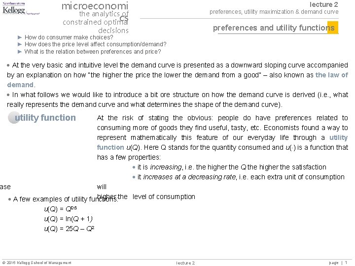
microeconomi the analytics of cs constrained optimal lecture 2 preferences, utility maximization & demand curve preferences and utility functions decisions ► How do consumer make choices? ► How does the price level affect consumption/demand? ► What is the relation between preferences and price? At the very basic and intuitive level the demand curve is presented as a downward sloping curve accompanied by an explanation on how “the higher the price the lower the demand from a good” – also known as the law of demand. In what follows we would like to introduce a bit ore structure on how the demand curve is derived (i. e. , what really represents the demand curve and what determines the shape of the demand curve). utility function At the risk of stating the obvious: people do have preferences related to consuming more of goods they find useful, tasty, etc. Economists found a way to represent mathematically this feature of our everyday life through a utility function u(Q). Here Q stands for the quantity consumed and u( ) is a function that has a few properties: it is increasing, i. e. the higher the Q the higher the satisfaction it increases at a decreasing rate, i. e. each extra unit of consumption ase will higher the level of consumption A few examples of utility functions: u(Q) = Q 0. 5 u(Q) = ln(Q + 1) u(Q) = 25 Q – Q 2 2016 Kellogg School of Management lecture 2 page | 1

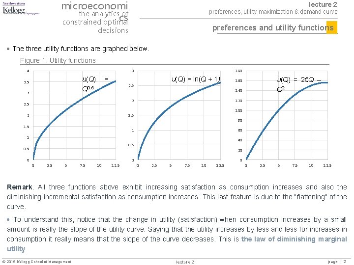
microeconomi the analytics of cs constrained optimal lecture 2 preferences, utility maximization & demand curve preferences and utility functions decisions The three utility functions are graphed below. Figure 1. Utility functions 4 3 u(Q) Q 0. 5 3 = 180 u(Q) = ln(Q + 1) 2. 5 140 2 2. 5 2 120 100 1. 5 80 1 60 1 0 40 0. 5 0 2. 5 5 7. 5 10 12. 5 0 u(Q) = 25 Q – Q 2 160 20 0 2. 5 5 7. 5 10 12. 5 Remark. All three functions above exhibit increasing satisfaction as consumption increases and also the diminishing incremental satisfaction as consumption increases. This last feature is due to the “flattening” of the curve. To understand this, notice that the change in utility (satisfaction) when consumption increases by a small amount is really the slope of the utility curve. Saying that the utility increases by less and less for increases in consumption it really means that the slope of the curve decreases. This is the law of diminishing marginal utility. 2016 Kellogg School of Management lecture 2 page | 2

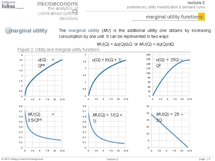
microeconomi the analytics of cs constrained optimal lecture 2 preferences, utility maximization & demand curve marginal utility functions decisions marginal utility The marginal utility (MU) is the additional utility one obtains by increasing consumption by one unit. It can be represented in two ways: MU(Q) = u(Q)/ Q or MU(Q) = du(Q)/d. Q Figure 2. Utility and marginal utility functions 3 4 u(Q) Q 0. 5 3 = 140 120 100 1. 5 80 1 1 60 40 0. 5 0 0 2. 5 5 7. 5 10 12. 5 0. 8 20 0 2. 5 5 7. 5 10 MU(Q) 0. 5/Q 0. 5 0. 6 0. 5 0. 4 0. 3 0. 2 0. 1 0 2. 5 5 2016 Kellogg School of Management 7. 5 10 12. 5 0 25 MU(Q) = 1/(Q + 1) 0. 6 0. 4 0 2. 5 5 7. 5 10 12. 5 30 0. 7 = 0 12. 5 0. 8 0. 7 u(Q) = 25 Q – Q 2 160 2 2 0 u(Q) = ln(Q + 1) 2. 5 0 180 MU(Q) = 25 – 2 Q 20 15 10 5 0 2. 5 5 7. 5 10 lecture 2 12. 5 0 0 2. 5 5 7. 5 10 12. 5 page | 3

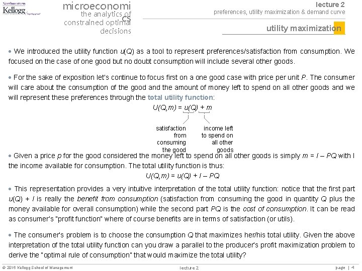
microeconomi the analytics of cs constrained optimal lecture 2 preferences, utility maximization & demand curve utility maximization decisions We introduced the utility function u(Q) as a tool to represent preferences/satisfaction from consumption. We focused on the case of one good but no doubt consumption will include several other goods. For the sake of exposition let’s continue to focus first on a one good case with price per unit P. The consumer will care about the consumption of the good and the amount of money left to spend on all other goods and we will represent these preferences through the total utility function: U(Q, m) = u(Q) + m satisfaction from consuming the good income left to spend on all other goods Given a price p for the good considered the money left to spend on all other goods is simply m = I – PQ with I the income available for consumption. The total utility function is thus: U(Q, m) = u(Q) + I – PQ This representation provides a very intuitive interpretation of the total utility function: notice that the first part u(Q) + I is really the benefit from consumption (satisfaction from consuming the good in quantity Q plus the money available for overall consumption) while the second part PQ is the cost of consumption. It can be read as consumer’s “profit function” where of course benefits are in terms of satisfaction (or utils). The consumer’s problem is to choose the consumption Q that maximizes her/his total utility. Given the above interpretation of the total utility function can you draw a parallel to the producer’s profit maximization problem to derive the “optimal rule of consumption” that would maximize the total utility? 2016 Kellogg School of Management lecture 2 page | 4

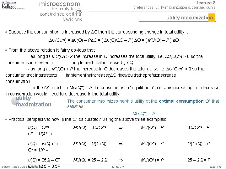
microeconomi the analytics of cs constrained optimal lecture 2 preferences, utility maximization & demand curve utility maximization decisions Suppose the consumption is increased by Q then the corresponding change in total utility is U(Q, m) = u(Q) – P Q = [ u(Q)/ Q – P ] Q = [ MU(Q) – P ] Q From the above relation is fairly obvious that: - as long as MU(Q) > P the increase in Q increases the total utility, i. e. U(Q, m) > 0 so the consumer is interested to implement that increase by Q - as long as MU(Q) < P the increase in Q decreases the total utility, i. e. U(Q, m) < 0 so the consumer isnot interestedto implementthatincreaseby Q, infactwouldratherprefertodecrease consumption - for the Q* for which MU(Q*) = P the consumer is in “equilibrium”, i. e. any increasing t or decrease in consumption would lead to a decrease in the total utility maximization The consumer maximizes her/his utility at the optimal consumption Q* that satisfies MU(Q*) = P Practical perspective: how is the Q* calculated? Using the above three examples: u(Q) = Q 0. 5 Q* = 1/(4 P 2) MU(Q) = 0. 5/Q 0. 5 MU(Q*) = P 0. 5/Q 0. 5 = P u(Q) = ln(Q +1) Q* = 1/P – 1 MU(Q) = 1/(1+Q) MU(Q*) = P 1/(1+Q) = P MU(Q) = 25 – 2 Q MU(Q*) = P 25 – 2 Q = P u(Q) = 25 Q – Q 2 2016 Kellogg School Q* of Management = 12. 5 – 0. 5 P lecture 2 page | 5

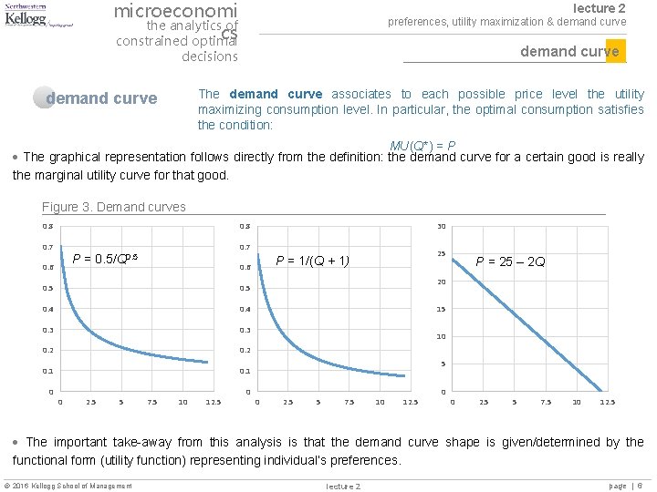
microeconomi the analytics of cs constrained optimal lecture 2 preferences, utility maximization & demand curve decisions The demand curve associates to each possible price level the utility maximizing consumption level. In particular, the optimal consumption satisfies the condition: demand curve MU(Q*) = P The graphical representation follows directly from the definition: the demand curve for a certain good is really the marginal utility curve for that good. Figure 3. Demand curves 0. 8 0. 7 P= 0. 6 0. 5/Q 0. 5 0. 4 0. 3 0. 2 0. 1 0 2. 5 5 7. 5 10 12. 5 0 25 P = 1/(Q + 1) 0. 6 0. 5 0 30 P = 25 – 2 Q 20 15 10 5 0 2. 5 5 7. 5 10 12. 5 0 0 2. 5 5 7. 5 10 12. 5 The important take-away from this analysis is that the demand curve shape is given/determined by the functional form (utility function) representing individual’s preferences. 2016 Kellogg School of Management lecture 2 page | 6

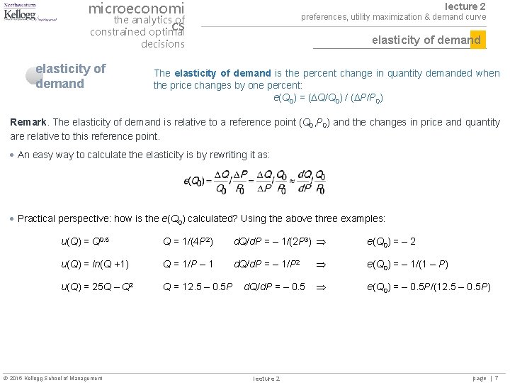
microeconomi the analytics of cs constrained optimal lecture 2 preferences, utility maximization & demand curve elasticity of demand decisions elasticity of demand The elasticity of demand is the percent change in quantity demanded when the price changes by one percent: e(Q 0) = ( Q/Q 0) / ( P/P 0) Remark. The elasticity of demand is relative to a reference point (Q 0, P 0) and the changes in price and quantity are relative to this reference point. An easy way to calculate the elasticity is by rewriting it as: Practical perspective: how is the e(Q 0) calculated? Using the above three examples: u(Q) = Q 0. 5 Q = 1/(4 P 2) d. Q/d. P = – 1/(2 P 3) u(Q) = ln(Q +1) Q = 1/P – 1 d. Q/d. P = – 1/P 2 u(Q) = 25 Q – Q 2 Q = 12. 5 – 0. 5 P 2016 Kellogg School of Management d. Q/d. P = – 0. 5 lecture 2 e(Q 0) = – 1/(1 – P) e(Q 0) = – 0. 5 P/(12. 5 – 0. 5 P) page | 7

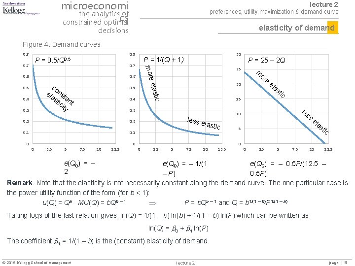
microeconomi the analytics of cs constrained optimal lecture 2 preferences, utility maximization & demand curve elasticity of demand decisions Figure 4. Demand curves 0. 8 P = 0. 5/Q 0. 5 0. 7 0. 6 0. 3 0. 4 lastic 0. 1 0 2. 5 5 7. 5 10 12. 5 0 0 2. 5 e 5 7. 5 el as tic le ss 10 less e 0. 2 0. 1 or 15 0. 3 0. 2 m 20 tic 0. 4 0. 5 P = 25 – 2 Q 25 elas co ela nst sti ant cit y 0. 5 0 more 0. 7 30 P = 1/(Q + 1) 10 12. 5 5 0 0 2. 5 5 7. 5 el 10 as tic 12. 5 e(Q 0) = – 2 e(Q 0) = – 1/(1 e(Q 0) = – 0. 5 P/(12. 5 – – P) 0. 5 P) Remark. Note that the elasticity is not necessarily constant along the demand curve. The one particular case is the power utility function of the form (for b < 1): u(Q) = Qb MU(Q) = b. Qb – 1 P = b. Qb – 1 and Q = b 1/(1 – b)P 1/(1 – b) Taking logs of the last relation gives ln(Q) = 1/(1 – b) ln(b) + 1/(1 – b) ln(P) which can be written as ln(Q) = 0 + 1 ln(P) The coefficient 1 = 1/(1 – b) is the (constant) elasticity of demand. 2016 Kellogg School of Management lecture 2 page | 8

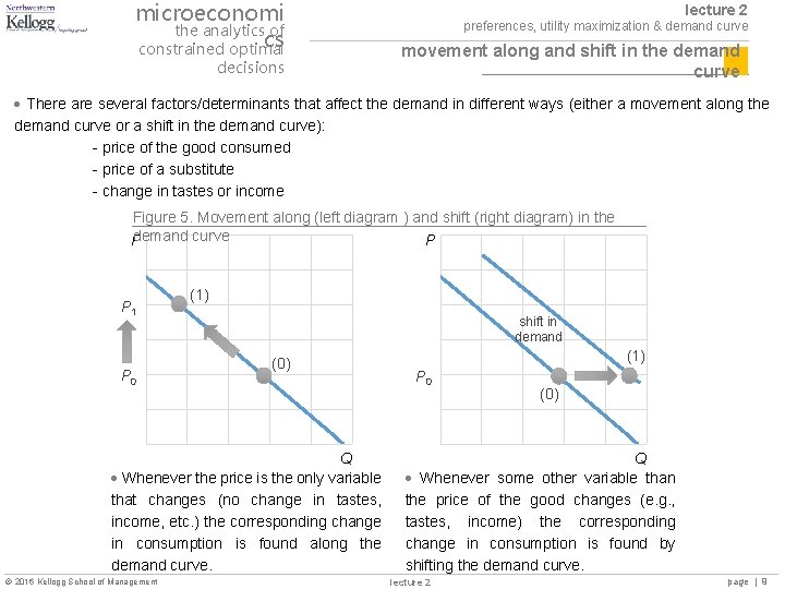
microeconomi the analytics of cs constrained optimal decisions lecture 2 preferences, utility maximization & demand curve movement along and shift in the demand curve There are several factors/determinants that affect the demand in different ways (either a movement along the demand curve or a shift in the demand curve): - price of the good consumed - price of a substitute - change in tastes or income Figure 5. Movement along (left diagram ) and shift (right diagram) in the demand curve P P P 1 P 0 (1) shift in demand (0) Q Whenever the price is the only variable that changes (no change in tastes, income, etc. ) the corresponding change in consumption is found along the demand curve. 2016 Kellogg School of Management (1) P 0 (0) Q Whenever some other variable than the price of the good changes (e. g. , tastes, income) the corresponding change in consumption is found by shifting the demand curve. lecture 2 page | 9

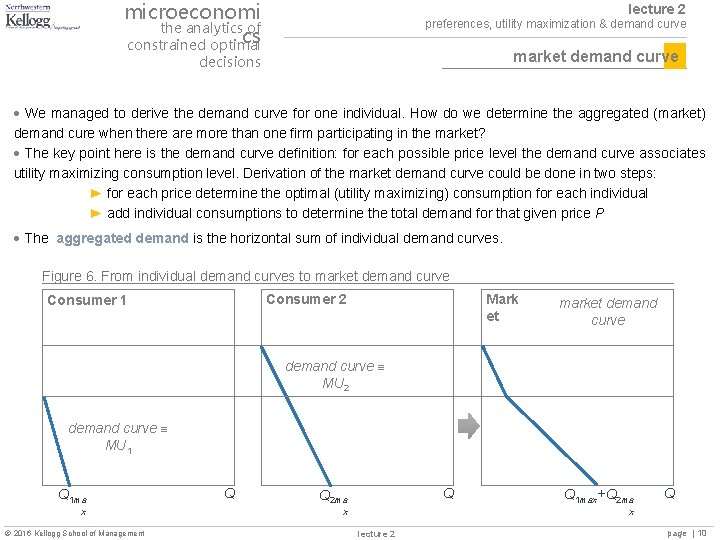
microeconomi the analytics of cs constrained optimal lecture 2 preferences, utility maximization & demand curve market demand curve decisions We managed to derive the demand curve for one individual. How do we determine the aggregated (market) demand cure when there are more than one firm participating in the market? The key point here is the demand curve definition: for each possible price level the demand curve associates utility maximizing consumption level. Derivation of the market demand curve could be done in two steps: ► for each price determine the optimal (utility maximizing) consumption for each individual ► add individual consumptions to determine the total demand for that given price P The aggregated demand is the horizontal sum of individual demand curves. Figure 6. From individual demand curves to market demand curve Consumer 2 Consumer 1 Mark et market demand curve MU 2 demand curve MU 1 Q 1 ma x 2016 Kellogg School of Management Q Q Q 2 ma Q 1 max+Q 2 ma Q x x lecture 2 page | 10

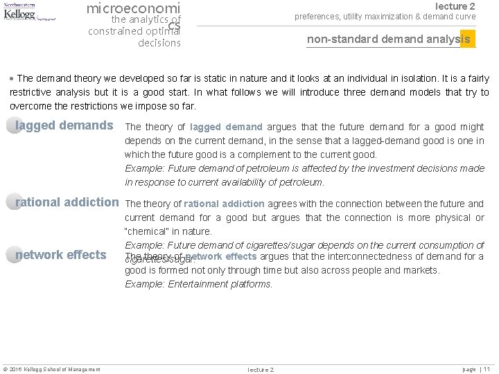
microeconomi the analytics of cs constrained optimal lecture 2 preferences, utility maximization & demand curve non-standard demand analysis decisions The demand theory we developed so far is static in nature and it looks at an individual in isolation. It is a fairly restrictive analysis but it is a good start. In what follows we will introduce three demand models that try to overcome the restrictions we impose so far. lagged demands The theory of lagged demand argues that the future demand for a good might depends on the current demand, in the sense that a lagged-demand good is one in which the future good is a complement to the current good. Example: Future demand of petroleum is affected by the investment decisions made in response to current availability of petroleum. rational addiction The theory of rational addiction agrees with the connection between the future and current demand for a good but argues that the connection is more physical or “chemical” in nature. Example: Future demand of cigarettes/sugar depends on the current consumption of The theory of network effects argues that the interconnectedness of demand for a cigarettes/sugar. good is formed not only through time but also across people and markets. Example: Entertainment platforms. network effects 2016 Kellogg School of Management lecture 2 page | 11

2016 Kellogg School of Management lecture 2 page | 12

microeconomi the analytics of cs constrained optimal lecture 2 preferences, utility maximization & demand curve network effects: the x. Box decisions Two friends live in two different cities and they both have one x. Box console. They pretty much have similar tastes and therefore like similar games. All games can be played either on an individual basis (vs. the “machine”) or in the network (vs. the “friend”) and all games are sold at the same price. i. No connection case. Currently the two cities are not connected through the internet and so all games are played individually. Both friends realize that they won’t buy any game is the price per game is above $1. If the games are given away for free (zero price) neither of the two friend would need more than 100 games. For prices in between $0 and $1 the demand is linear. ► What are the individual demand functions? ► What is the market demand? ii. Connection case. Finally the two cities get connected through the internet and now all games can be played between “friends”. However, this new feature changes slightly the preferences for games: both friends are willing to buy games for up to a price of $1. 5 and they would like to have about 200 games if they could get them for free. For prices in between $0 and $1. 5 the demand is linear. ► What are the new individual demand functions? ► What is the market demand? iii. Network effect. Compare the two results above. Why the difference? 2016 Kellogg School of Management lecture 2 page | 13

microeconomi the analytics of cs constrained optimal lecture 2 preferences, utility maximization & demand curve demand for pay-per-view events decisions A known TV cable network offers a pay-per-view option for its currently 1, 000 subscribers that will give access to a Saturday Night Live sport event. The TV provider will announce a price P for the pay-per-view event, each of the 1, 000 subscribers will decide whether to pay the price P (in which case she/he will enjoy the SNL sport event) or not. Each subscriber has a maximum price level, called a reservation price level RP, that she/he is willing to pay: if P > RP the subscriber will not take the pay-per-view offer. Assume here that all RPi are between $0 and $1. i. Known reservation prices. Let’s start with the simple case in which the TV provider knows the reservation price RPi for each subscriber i = 1… 1, 000 (provided in the excel file “PPV. xlsx”) ► Pick one subscriber and draw her/his demand curve. ► What is the market demand? (include all 1, 000 subscribers) ii. Unknown reservation prices. The more realistic scenario is the one in which the TV channel does not have precise information about the RPi, however it estimates that each RPi can be any value between $0 and $1 with equal probability. In other words RPi is uniformly distributed between $0 and $1. ► How would you determine the market demand? Here consider the following hint: for each price level determine the expected number of subscribers – this is the expected market demand. 2016 Kellogg School of Management lecture 2 page | 14