Session on Assessment of Food Exposure Food Exposure

Session on Assessment of Food Exposure

Food Exposure William O. Smith, Ph. D. Chemist Health Effects Division Office of Pesticide Programs 2

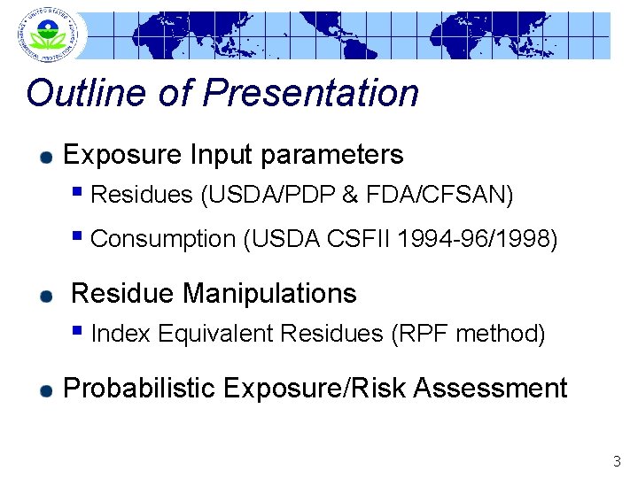
Outline of Presentation Exposure Input parameters § Residues (USDA/PDP & FDA/CFSAN) § Consumption (USDA CSFII 1994 -96/1998) Residue Manipulations § Index Equivalent Residues (RPF method) Probabilistic Exposure/Risk Assessment 3

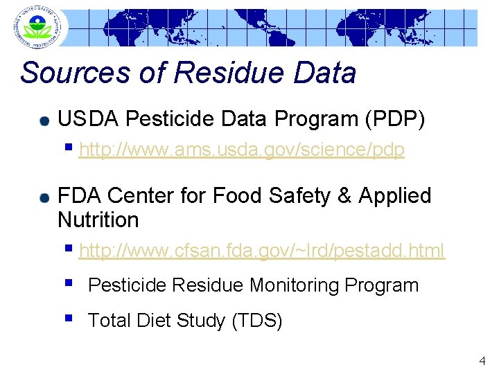
Sources of Residue Data USDA Pesticide Data Program (PDP) § http: //www. ams. usda. gov/science/pdp FDA Center for Food Safety & Applied Nutrition § http: //www. cfsan. fda. gov/~lrd/pestadd. html § Pesticide Residue Monitoring Program § Total Diet Study (TDS) 4

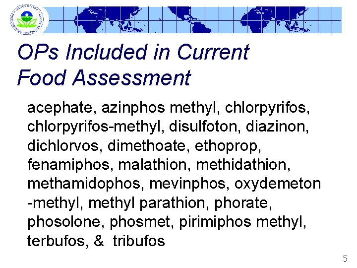
OPs Included in Current Food Assessment acephate, azinphos methyl, chlorpyrifos-methyl, disulfoton, diazinon, dichlorvos, dimethoate, ethoprop, fenamiphos, malathion, methidathion, methamidophos, mevinphos, oxydemeton -methyl, methyl parathion, phorate, phosolone, phosmet, pirimiphos methyl, terbufos, & tribufos 5

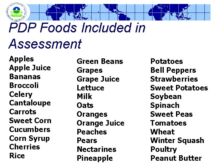
PDP Foods Included in Assessment Apples Apple Juice Bananas Broccoli Celery Cantaloupe Carrots Sweet Corn Cucumbers Corn Syrup Cherries Rice Green Beans Grape Juice Lettuce Milk Oats Orange Juice Peaches Pears Nectarines Pineapple Potatoes Bell Peppers Strawberries Sweet Potatoes Soybean Spinach Sweet Peas Tomatoes Wheat Winter Squash Poultry Peanut Butter

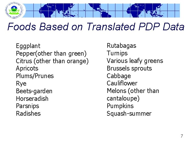
Foods Based on Translated PDP Data Eggplant Pepper(other than green) Citrus (other than orange) Apricots Plums/Prunes Rye Beets-garden Horseradish Parsnips Radishes Rutabagas Turnips Various leafy greens Brussels sprouts Cabbage Cauliflower Melons (other than cantaloupe) Pumpkins Squash-summer 7

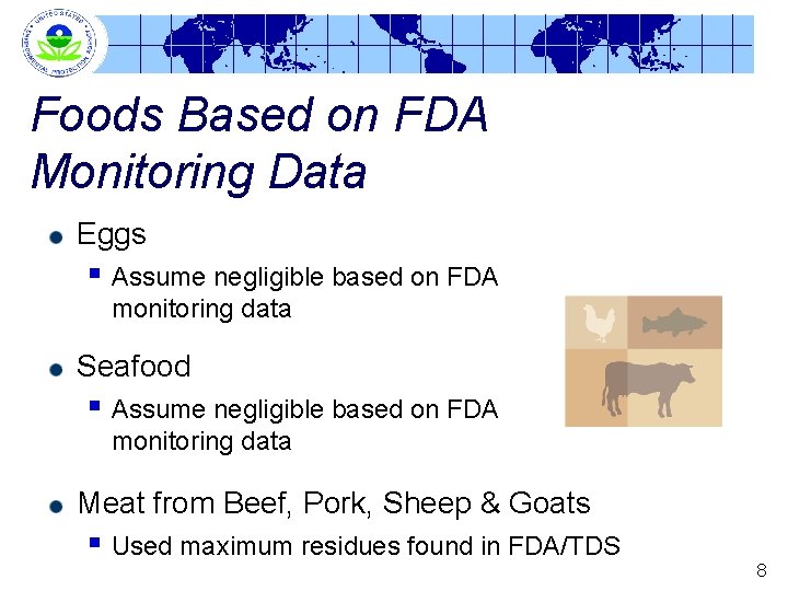
Foods Based on FDA Monitoring Data Eggs § Assume negligible based on FDA monitoring data Seafood § Assume negligible based on FDA monitoring data Meat from Beef, Pork, Sheep & Goats § Used maximum residues found in FDA/TDS 8

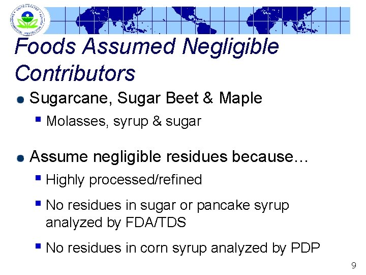
Foods Assumed Negligible Contributors Sugarcane, Sugar Beet & Maple § Molasses, syrup & sugar Assume negligible residues because… § Highly processed/refined § No residues in sugar or pancake syrup analyzed by FDA/TDS § No residues in corn syrup analyzed by PDP 9

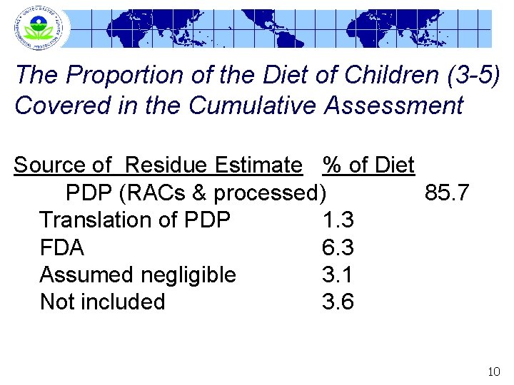
The Proportion of the Diet of Children (3 -5) Covered in the Cumulative Assessment Source of Residue Estimate % of Diet PDP (RACs & processed) 85. 7 Translation of PDP 1. 3 FDA 6. 3 Assumed negligible 3. 1 Not included 3. 6 10

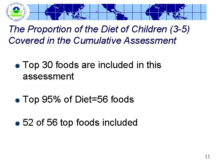
The Proportion of the Diet of Children (3 -5) Covered in the Cumulative Assessment Top 30 foods are included in this assessment Top 95% of Diet=56 foods 52 of 56 top foods included 11

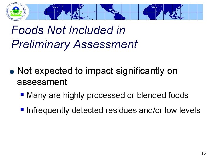
Foods Not Included in Preliminary Assessment Not expected to impact significantly on assessment § Many are highly processed or blended foods § Infrequently detected residues and/or low levels 12

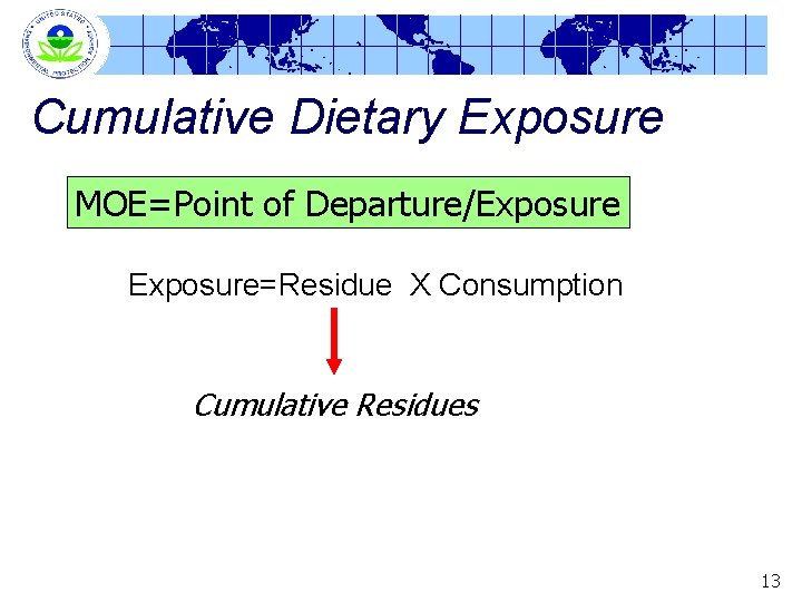
Cumulative Dietary Exposure MOE=Point of Departure/Exposure=Residue X Consumption Cumulative Residues 13

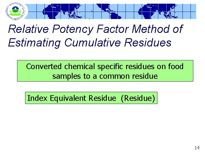
Relative Potency Factor Method of Estimating Cumulative Residues Converted chemical specific residues on food samples to a common residue Index Equivalent Residue (Residue) 14

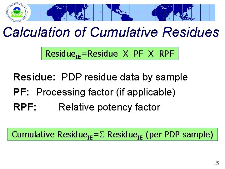
Calculation of Cumulative Residues Residue. IE=Residue X PF X RPF Residue: PDP residue data by sample PF: Processing factor (if applicable) RPF: Relative potency factor Cumulative Residue. IE=S Residue. IE (per PDP sample) 15

Residue Inputs for Cumulative Assessment Distributions of cumulative residues OR Average cumulative residues for highly blended foods 16

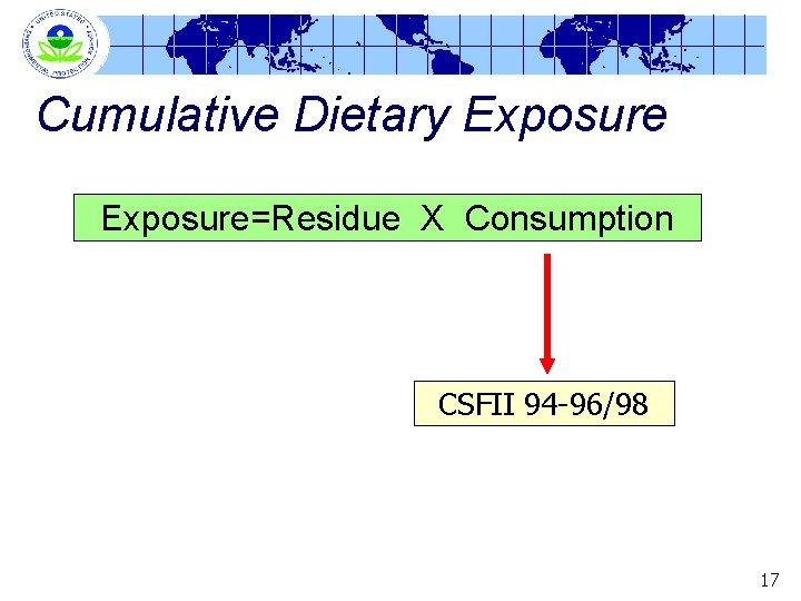
Cumulative Dietary Exposure=Residue X Consumption CSFII 94 -96/98 17

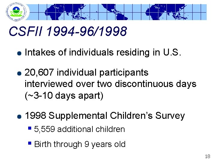
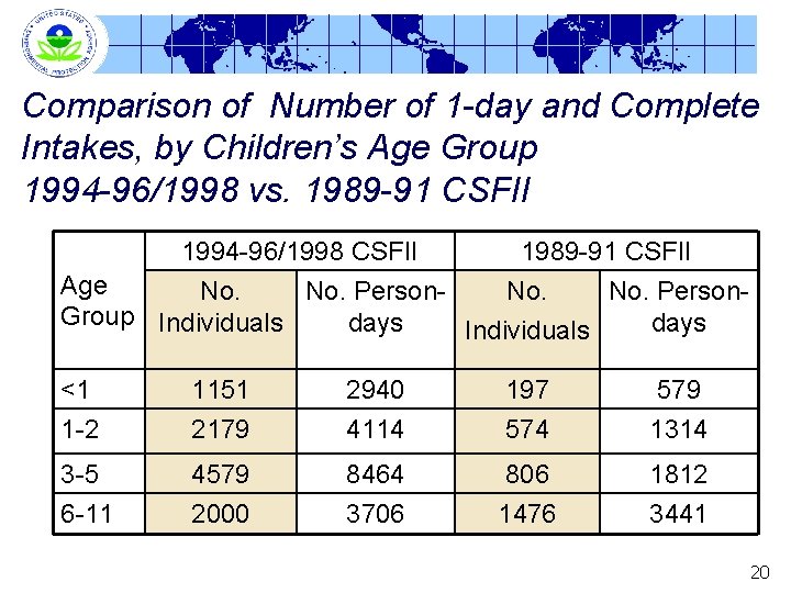
CSFII 1994 -96/1998 Intakes of individuals residing in U. S. 20, 607 individual participants interviewed over two discontinuous days (~3 -10 days apart) 1998 Supplemental Children’s Survey § 5, 559 additional children § Birth through 9 years old 18

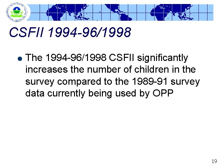
CSFII 1994 -96/1998 The 1994 -96/1998 CSFII significantly increases the number of children in the survey compared to the 1989 -91 survey data currently being used by OPP 19

Comparison of Number of 1 -day and Complete Intakes, by Children’s Age Group 1994 -96/1998 vs. 1989 -91 CSFII 1994 -96/1998 CSFII 1989 -91 CSFII Age No. No. Person. Group Individuals days Individuals <1 1 -2 1151 2179 2940 4114 197 574 579 1314 3 -5 6 -11 4579 2000 8464 3706 806 1476 1812 3441 20

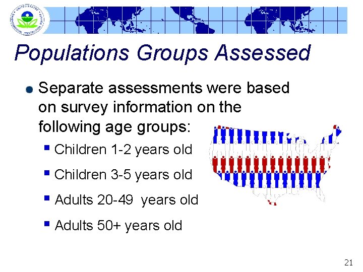
Populations Groups Assessed Separate assessments were based on survey information on the following age groups: § Children 1 -2 years old § Children 3 -5 years old § Adults 20 -49 years old § Adults 50+ years old 21

Exposure Assessment Models DEEM™ and Calendex™ were used to estimate cumulative food exposure and risk The use of Calendex™ and related issues will be discussed next by David Miller 22

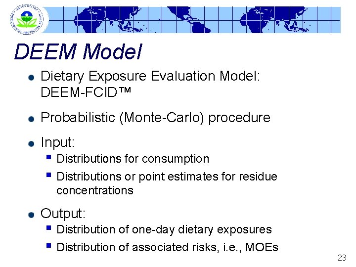
DEEM Model Dietary Exposure Evaluation Model: DEEM-FCID™ Probabilistic (Monte-Carlo) procedure Input: § Distributions for consumption § Distributions or point estimates for residue concentrations Output: § Distribution of one-day dietary exposures § Distribution of associated risks, i. e. , MOEs 23

Dietary Exposure Evaluation Model DEEM-FCID™ Uses EPA's Food Commodity Intake Database Commodity definitions are based on EPA's Food Commodity Vocabulary Recipes for relating foods consumed to raw commodities are publicly available 24

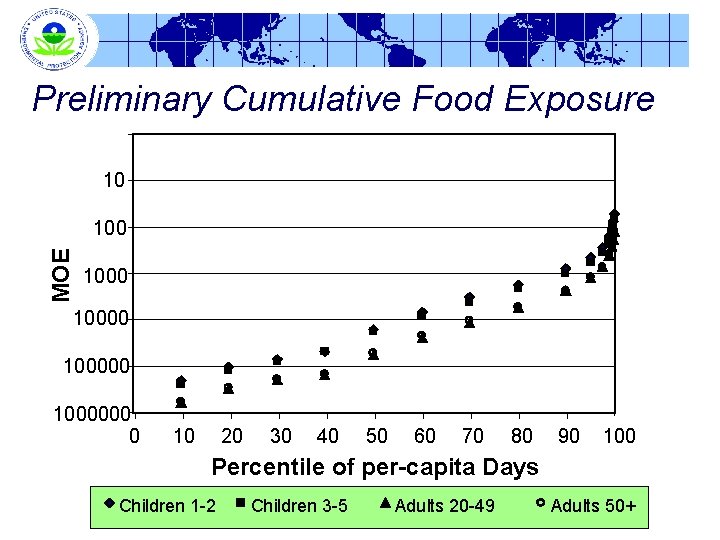
Preliminary Cumulative Food Exposure 10 MOE 100000 1000000 0 10 20 30 40 50 60 70 80 90 100 Percentile of per-capita Days Children 1 -2 Children 3 -5 Adults 20 -49 Adults 50+

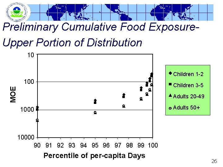
Preliminary Cumulative Food Exposure. Upper Portion of Distribution 10 Children 1 -2 100 MOE Children 3 -5 Adults 20 -49 Adults 50+ 10000 90 91 92 93 94 95 96 97 98 99 100 Percentile of per-capita Days 26

Preliminary Cumulative Exposure Assessment Margin of Exposure (MOE) at Upper-End of Distribution Percentile 90 th 95 th 97. 5 th 99. 9 th Children 1 -2 800 Children 3 -5 994 454 562 280 348 160 196 108 133 51 62 Adults 20 -49 2415 1280 Adults 50+ 2321 1228 755 720 415 393 281 264 127 125 MOE = POD/exposure; POD = 0. 08 mg/kg body wt/day 27

Preliminary Final Work to be completed… Further refinements to inputs Interpretation of results 28

Potential Effects of Input Assumptions & Refinements on the Assessment Translation of PDP residue data to other foods Use of processing factors to estimate residues in processed food forms (cooked, dried, juices, etc. ) 29

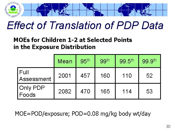
Effect of Translation of PDP Data MOEs for Children 1 -2 at Selected Points in the Exposure Distribution Full Assessment Only PDP Foods Mean 95 th 99. 9 th 2001 457 160 110 52 2082 470 165 114 53 MOE=POD/exposure; POD=0. 08 mg/kg body wt/day 30

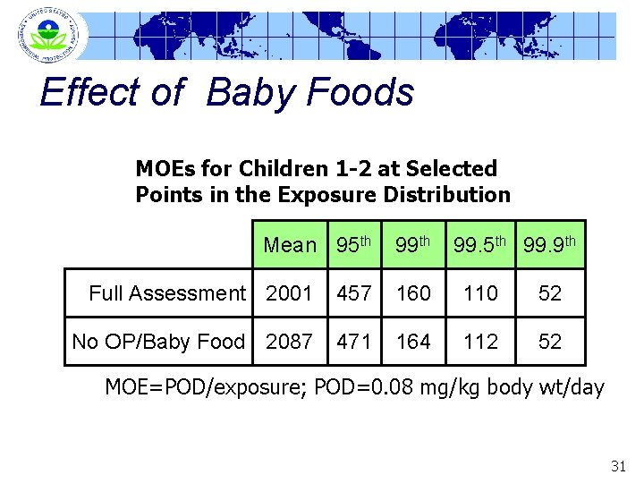
Effect of Baby Foods MOEs for Children 1 -2 at Selected Points in the Exposure Distribution Mean 95 th 99. 9 th Full Assessment 2001 457 160 110 52 No OP/Baby Food 2087 471 164 112 52 MOE=POD/exposure; POD=0. 08 mg/kg body wt/day 31

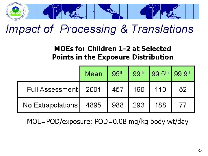
Impact of Processing & Translations MOEs for Children 1 -2 at Selected Points in the Exposure Distribution Mean 95 th 99. 9 th Full Assessment 2001 457 160 110 52 No Extrapolations 4895 988 293 188 77 MOE=POD/exposure; POD=0. 08 mg/kg body wt/day 32

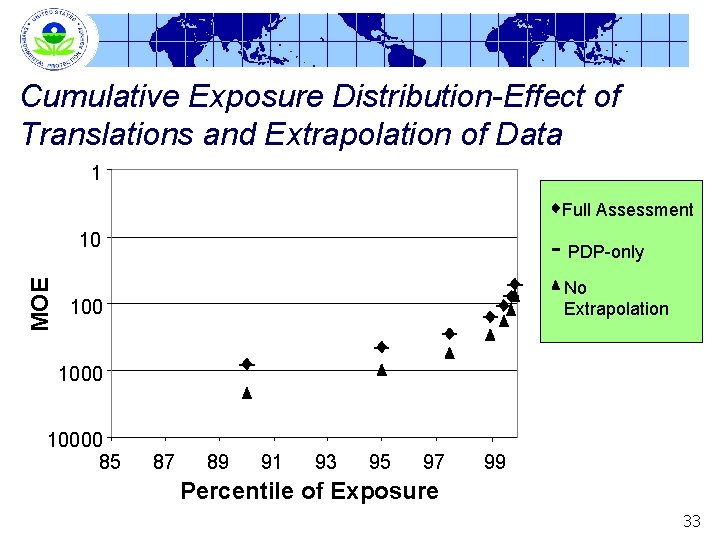
Cumulative Exposure Distribution-Effect of Translations and Extrapolation of Data 1 Full Assessment MOE 10 PDP-only No Extrapolation 10000 85 87 89 91 93 95 97 99 Percentile of Exposure 33

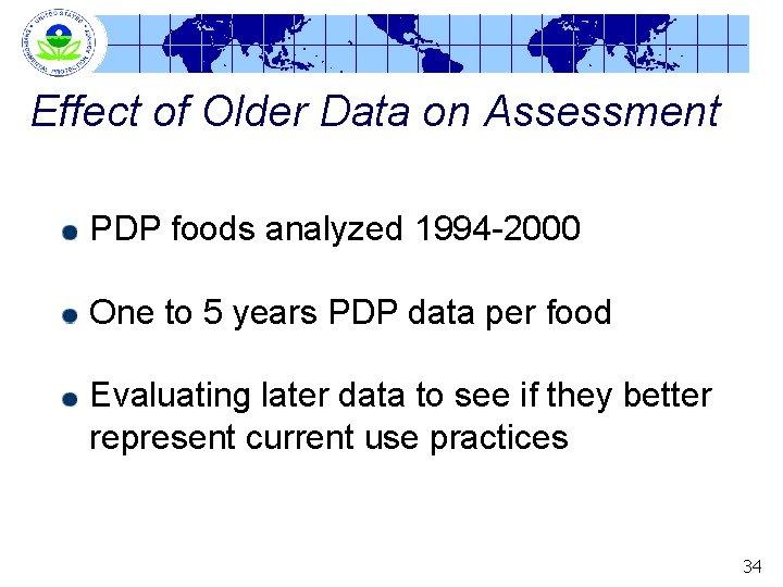
Effect of Older Data on Assessment PDP foods analyzed 1994 -2000 One to 5 years PDP data per food Evaluating later data to see if they better represent current use practices 34

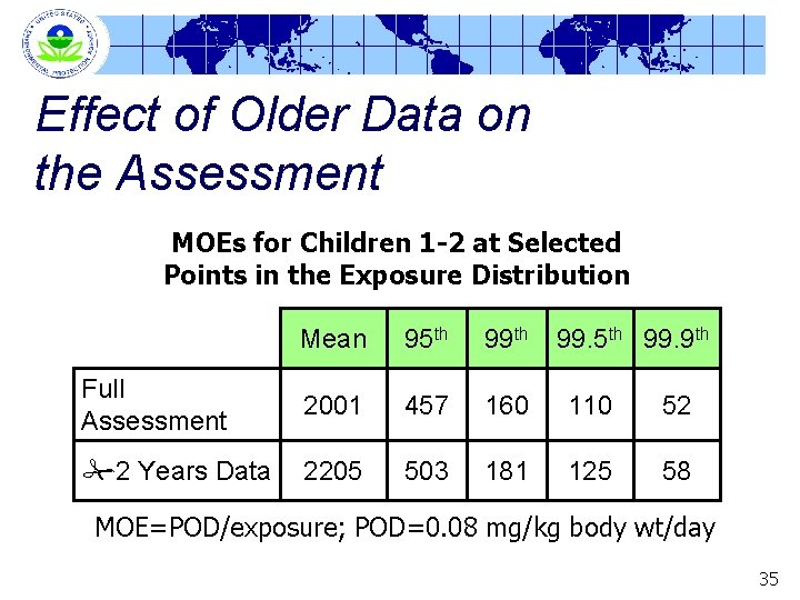
Effect of Older Data on the Assessment MOEs for Children 1 -2 at Selected Points in the Exposure Distribution Mean 95 th 99. 9 th Full Assessment 2001 457 160 110 52 2 Years Data 2205 503 181 125 58 MOE=POD/exposure; POD=0. 08 mg/kg body wt/day 35

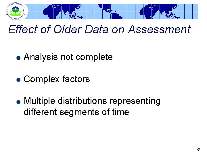
Effect of Older Data on Assessment Analysis not complete Complex factors Multiple distributions representing different segments of time 36

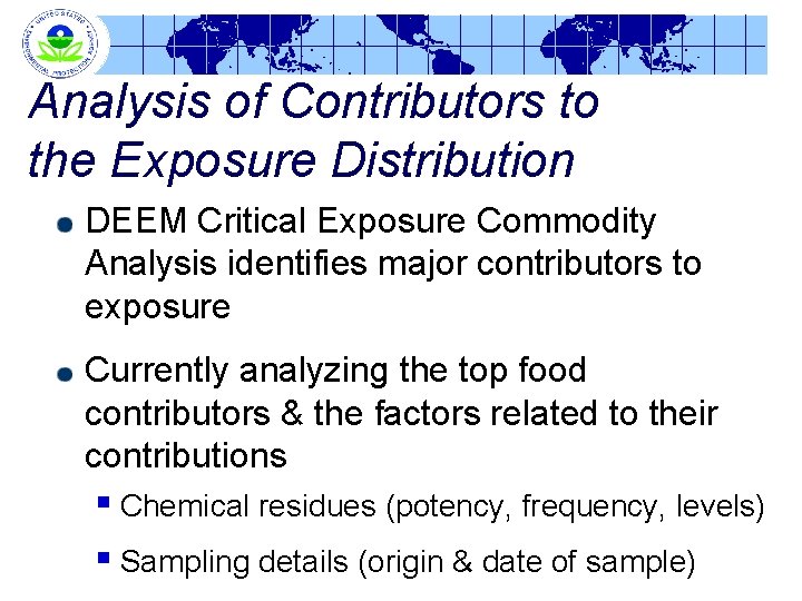
Analysis of Contributors to the Exposure Distribution DEEM Critical Exposure Commodity Analysis identifies major contributors to exposure Currently analyzing the top food contributors & the factors related to their contributions § Chemical residues (potency, frequency, levels) § Sampling details (origin & date of sample)

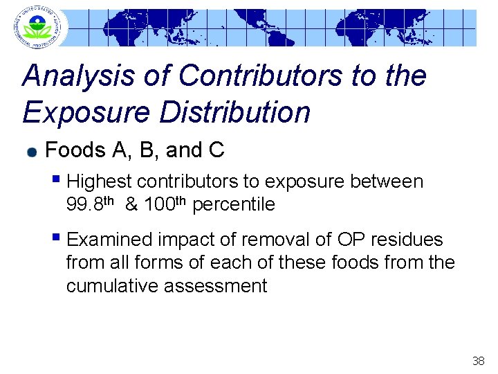
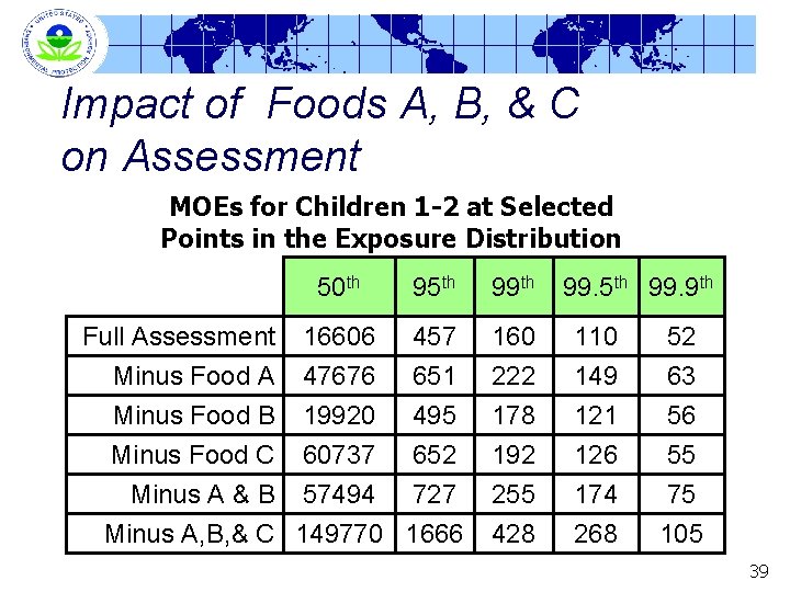
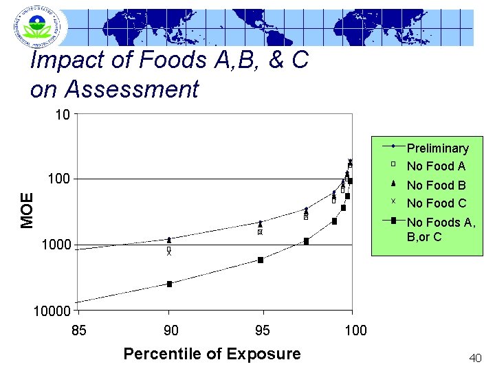
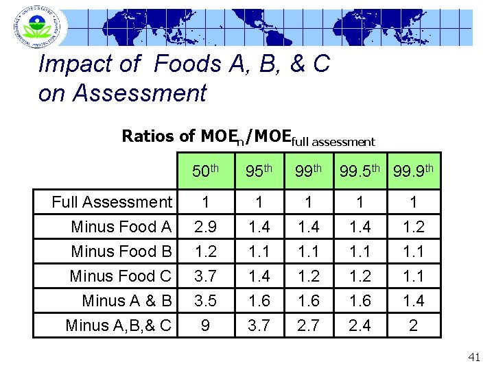
Analysis of Contributors to the Exposure Distribution Foods A, B, and C § Highest contributors to exposure between 99. 8 th & 100 th percentile § Examined impact of removal of OP residues from all forms of each of these foods from the cumulative assessment 38

Impact of Foods A, B, & C on Assessment MOEs for Children 1 -2 at Selected Points in the Exposure Distribution 50 th 95 th 99. 9 th Full Assessment Minus Food A 16606 47676 457 651 160 222 110 149 52 63 Minus Food B Minus Food C 19920 60737 495 652 178 192 121 126 56 55 Minus A & B 57494 727 Minus A, B, & C 149770 1666 255 428 174 268 75 105 39

Impact of Foods A, B, & C on Assessment 10 Preliminary No Food A 100 MOE No Food B No Food C No Foods A, B, or C 10000 85 90 95 Percentile of Exposure 100 40

Impact of Foods A, B, & C on Assessment Ratios of MOEn/MOEfull assessment 50 th 95 th 99. 9 th Full Assessment Minus Food A Minus Food B Minus Food C 1 2. 9 1. 2 3. 7 1 1. 4 1. 1 1. 2 1. 1 Minus A & B Minus A, B, & C 3. 5 9 1. 6 3. 7 1. 6 2. 4 1. 4 2 41

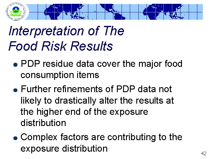
Interpretation of The Food Risk Results PDP residue data cover the major food consumption items Further refinements of PDP data not likely to drastically alter the results at the higher end of the exposure distribution Complex factors are contributing to the exposure distribution 42

Calendar-Based Exposure Assessment Calendex™ was used to estimate cumulative exposure from food, water, and residential uses as a series of daily exposure distributions for a year This time-series food exposure assessment and related issues will be discussed next by David Miller 43

Time-Frame Considerations David Miller Chemist (USPHS) Health Effects Division 44

Outline of Presentation Introduction/Background information DEEM(FCID)™ vs. DEEM(FCID)/Calendex™ Time-Frame Considerations Modes in which Calendex™ can be used for a cumulative risk assessment § Consecutive daily estimates § Rolling (or sliding) time-frame Strengths and limitations of these modes Questions for the SAP 45

Points to Remember… Presentation will not review step-by-step mechanics of DEEM(FCID)/Calendex™ algorithms: § DEEM/Calendex™ reviewed in previous SAPs Presentation concentrates on exposure through food § Principles apply to all routes No decision has been made on an appropriate MOE or threshold percentile for regulation 46

Introduction DEEM(FCID)/Calendex™ provides a probabilistic assessment of exposures through food, water, and residential pathways § DEEM(FCID)/Calendex™ incorporates concept of a Calendar to evaluate aggregate or cumulative exposures • Time-based approach § Calendar-based approach looks at each individual day of the year § Calendar-based approach allows appropriate “temporal matching” of exposures through food, drinking water, and residential pathways • Temporal aspect of exposure important for OP’s due to expected seasonal use-patterns 47

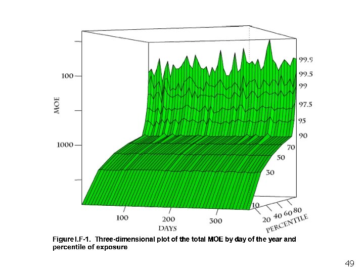
Introduction Calendex™ uses probabilistic techniques to appropriately combine exposures from the food, water, and residential pathways in a manner which incorporates: § § § probabilities of exposure, use and application practices, human activity patterns, etc. and considers their associated seasonality and timing Result is a collection (or distribution) of aggregate exposures (food, residential, and drinking water combined) for each day of the year for the relevant region These exposures can be plotted as a “time-line” or profile of daily exposures for any given percentile in the distribution

49

How Does DEEM(FCID)/Calendex™ differ from DEEM(FCID)™? DEEM(FCID)™ analysis assesses exposure from food alone without respect to timing/seasonality issues § Randomly matches reported food consumption, by individual, with residue data • No time component § Result is a single distribution of exposures and a single-valued estimate of risk at any given percentile of exposure 50

How Does DEEM(FCID)/Calendex™ differ from DEEM(FCID)™? In an aggregate or cumulative assessment in which pathways are combined, timing considerations are important DEEM(FCID)/Calendex™ performs analysis in a manner in which timing considerations are incorporated § Does this by performing separate analyses for each day of the year § Result is 365 separate distributions of exposures for each of the day of the year § Exposures at any given percentile can be plotted as a time-based exposure profile 51

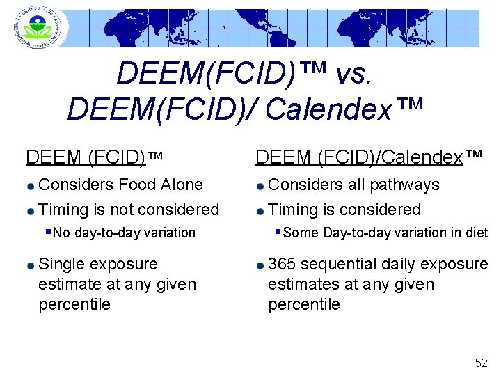
DEEM(FCID)™ vs. DEEM(FCID)/ Calendex™ DEEM (FCID)™ Considers Food Alone Timing is not considered DEEM (FCID)/Calendex™ Considers all pathways Timing is considered §No day-to-day variation §Some Day-to-day variation in diet Single exposure estimate at any given percentile 365 sequential daily exposure estimates at any given percentile 52

Time-Frame Considerations Important to consider how estimated exposure is compared with toxicity endpoint § Toxicity endpoint in PCRA is based on BMD 10 which reflects multi-day dosing studies 53

Time-Frame Considerations September 2001 SAP Meeting considered this issue of how to compare time component of toxicity endpoints and exposure: § CRA should ideally compare toxicity endpoints and exposure durations of same time-frame § To the extent possible, comparison should take into account the pattern of human exposure 54

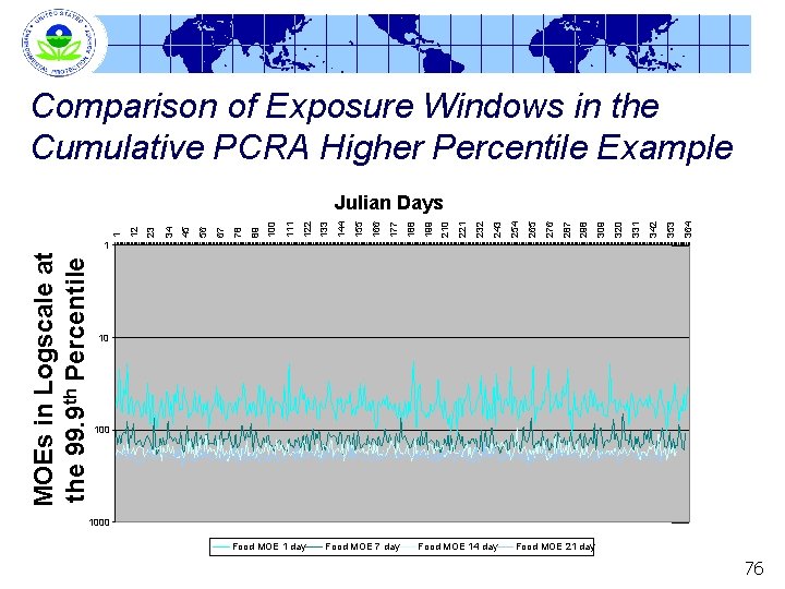
Time-Frame Considerations DEEM/Calendex™ program can perform analysis using a variety of time-frames This presentation considers two specific modes of analysis: § Single Consecutive daily estimates § Rolling (or sliding) time-frame Examples here are illustrative only 55

Single (Consecutive) Day Analysis Single Consecutive Day Option § Separate independent exposure and risk (MOE) estimates made for each day of the year § Estimates are arrayed chronologically into an exposure time line for any selected percentile and graphed • These represent independent, daily estimates of risk on each day of the year – Not necessarily the same individual on consecutive days 56

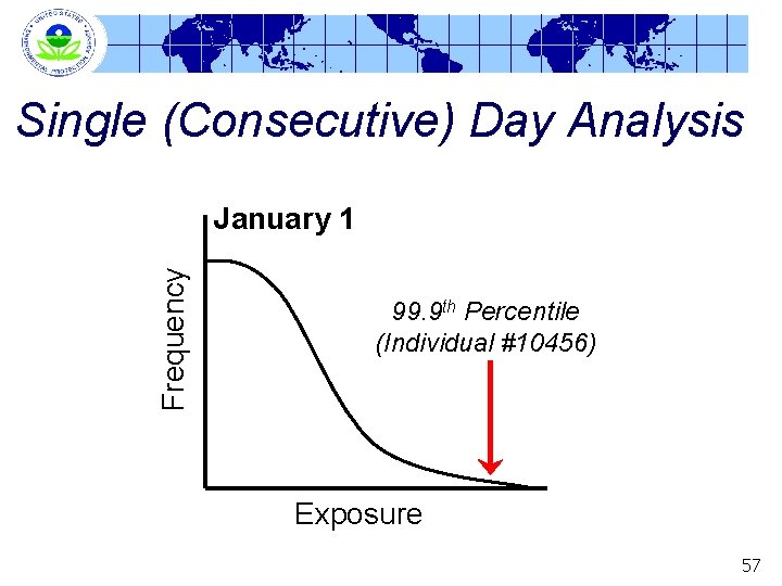
Single (Consecutive) Day Analysis Frequency January 1 99. 9 th Percentile (Individual #10456) Exposure 57

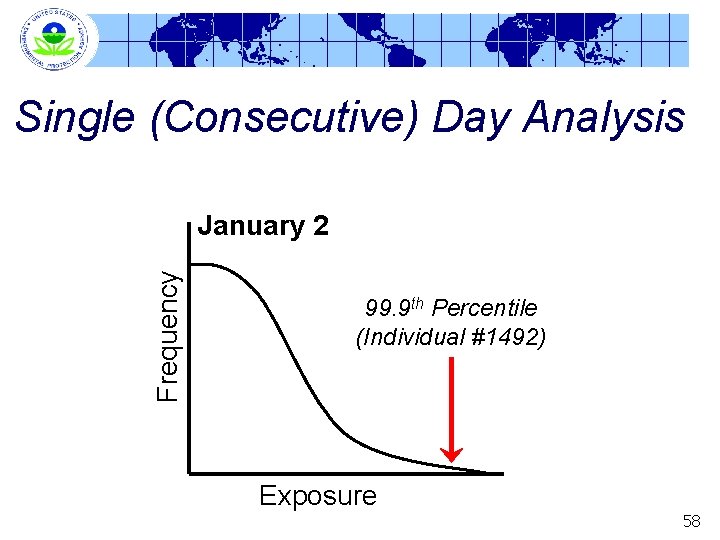
Single (Consecutive) Day Analysis Frequency January 2 99. 9 th Percentile (Individual #1492) Exposure 58

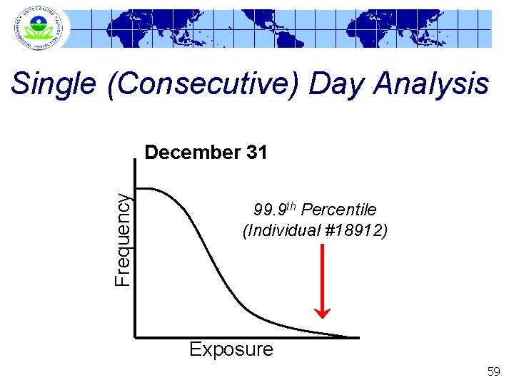
Single (Consecutive) Day Analysis Frequency December 31 99. 9 th Percentile (Individual #18912) Exposure 59

Single (Consecutive) Day Analysis Plot, for each day, a fixed population exposure percentile (e. g. , 99. 9 th) Resulting time-based exposure profile represents 99. 9 th percentile exposure for each day of the year § each day of year considered independently 60

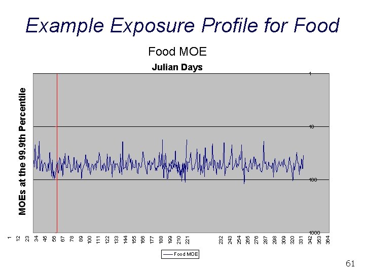
364 353 MOEs at the 99. 9 th Percentile Julian Days 342 331 320 309 298 287 276 265 254 243 232 221 210 199 188 177 166 155 144 133 122 111 100 89 78 67 56 45 34 23 12 1 Example Exposure Profile for Food MOE 1 10 1000 Food MOE 61

Example Exposure Profile for Food On Day 31, the MOEF at the 99. 9 th percentile is 58 § Translation: • Exposure to the 99. 9 th percentile individual on Day 31 is 58 times lower than the POD On Day 32, the MOEF at the 99. 9 th percentile is 66 § Translation: • Exposure to the 99. 9 th percentile individual on Day 32 is 66 times lower than the POD – This is likely to be a different individual than the 99. 9 th percentile individual on Day 31 62

Pros and Cons for Single-Day Based Estimate Pros: § § Easier to identify risk contributors Health protective • unlikely to underestimate average exposure over multiple days Cons: § Point of Departure is based on multi-day exposure • Relevance of comparing a series of single-day exposures to multi-day endpoint § Consecutive daily estimates are likely to overestimate multi-day exposures to an individual (at higher percentiles) • e. g. , not possible to interpret extended series of elevated exposures on consecutive days as representing extended period of exposure to the same individual. 63

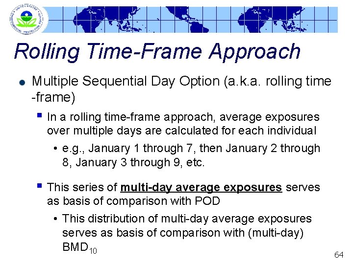
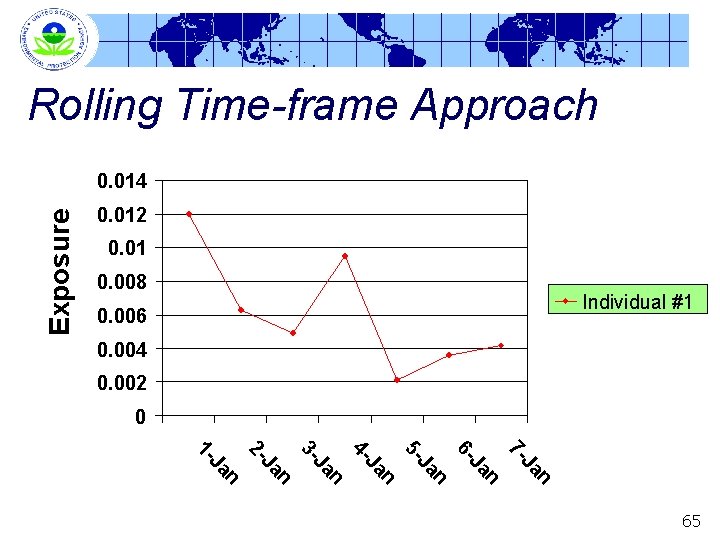
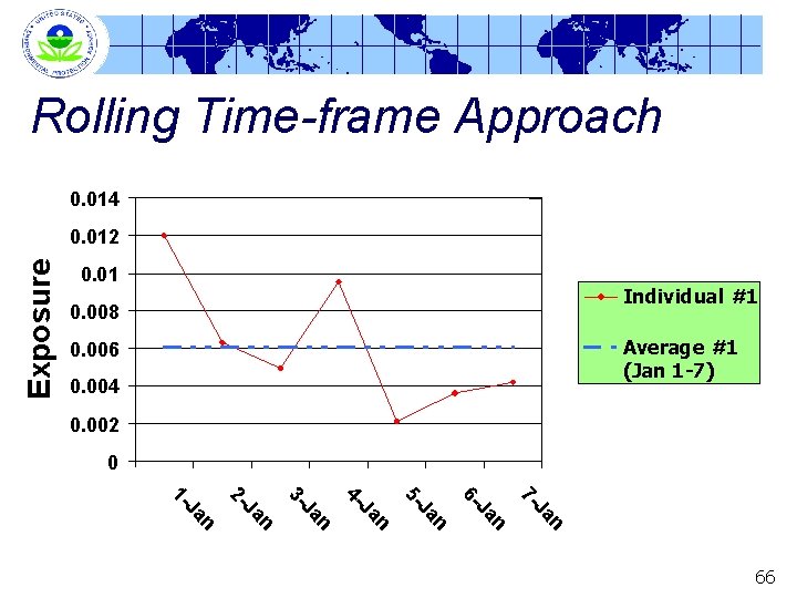
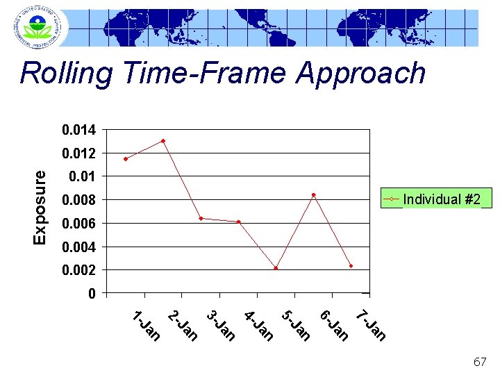
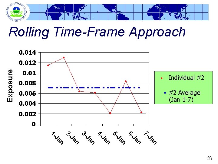
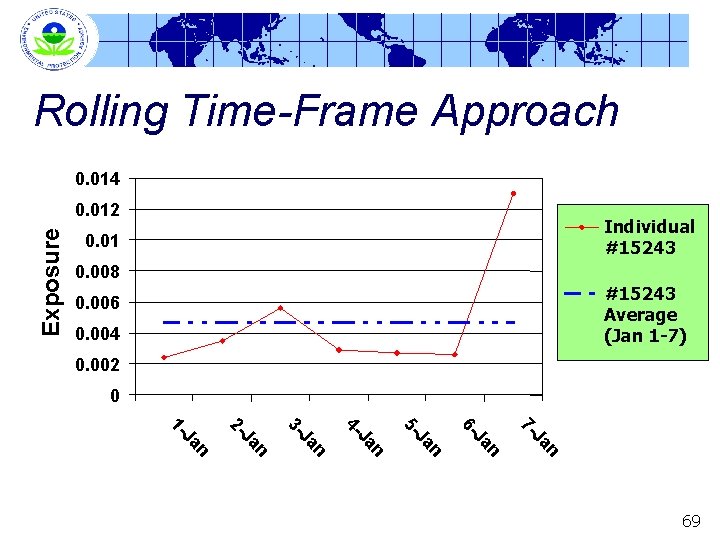
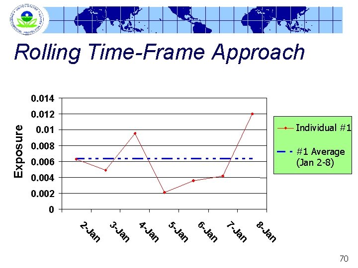
Rolling Time-Frame Approach Multiple Sequential Day Option (a. k. a. rolling time -frame) § In a rolling time-frame approach, average exposures over multiple days are calculated for each individual • e. g. , January 1 through 7, then January 2 through 8, January 3 through 9, etc. § This series of multi-day average exposures serves as basis of comparison with POD • This distribution of multi-day average exposures serves as basis of comparison with (multi-day) BMD 10 64

Rolling Time-frame Approach Exposure 0. 014 0. 012 0. 01 0. 008 Individual #1 0. 006 0. 004 0. 002 0 n Ja 7 - n Ja 6 - n Ja 5 - n Ja 4 - n Ja 3 - n Ja 2 - n Ja 1 - 65

Rolling Time-frame Approach 0. 014 Exposure 0. 012 0. 01 Individual #1 0. 008 Average #1 (Jan 1 -7) 0. 006 0. 004 0. 002 0 n Ja 7 - n Ja 6 - n Ja 5 - n Ja 4 - n Ja 3 - n Ja 2 - n Ja 1 - 66

Rolling Time-Frame Approach 0. 014 Exposure 0. 012 0. 01 Individual #2 0. 008 0. 006 0. 004 0. 002 0 n Ja 7 - n Ja 6 - n Ja 5 - n Ja 4 - n Ja 3 - n Ja 2 - n Ja 1 - 67

Rolling Time-Frame Approach 0. 014 Exposure 0. 012 0. 01 Individual #2 0. 008 #2 Average (Jan 1 -7) 0. 006 0. 004 0. 002 0 1 J an 2 - Ja n 3 - Ja n 4 - Ja n 5 - Ja n 6 - Ja n 7 - Ja n 68

Rolling Time-Frame Approach 0. 014 Exposure 0. 012 Individual #15243 0. 01 0. 008 #15243 Average (Jan 1 -7) 0. 006 0. 004 0. 002 0 n Ja 7 - n Ja 6 - n Ja 5 - n Ja 4 - n Ja 3 - n Ja 2 - n Ja 1 - 69

Rolling Time-Frame Approach 0. 014 Exposure 0. 012 Individual #1 0. 008 #1 Average (Jan 2 -8) 0. 006 0. 004 0. 002 0 n Ja 8 - n Ja 7 - n Ja 6 - n Ja 5 - n Ja 4 - n Ja 3 - n Ja 2 - 70

Pros and Cons for Rolling. Average Based Estimates Pros: § Incorporate variability in exposure for an individual across multiple days § Likely to provide a more realistic estimate of exposures across multiple days § Flexible with respect to matching time-frame associated with POD 71

Pros and Cons for Rolling. Average Based Estimates Cons: § USDA’s CSFII does not provide consumption data across the multiple consecutive days which would be of interest • Limited to two days of reported intake • Two days are not consecutive (3 -10 days apart) • Multi-day average exposure for any individual uses only two days of reported consumption data for that individual – and repeats these (randomly) through the time-frame of interest § No “longitudinal” residue data is available 72

Issues: Food Consumption Any consecutive day period of interest for an individual will contain a series of repeated diets which tend to underestimate variability § This will tend to overstate potential exposure at upper tails of distribution to the extent that reported diets (food choices) are associated with higher exposure 73

Issues: Residues Since residue values are drawn (anew) at random for each day during the time-frame of interest, true correlations that may exist between residues on subsequent days may not be accurately reflected § This will tend to understate potential exposure at the upper tails of the distribution to the extent that an individual’s exposure is associated with pesticide residue concentrations • Juices • Bags of Produce 74

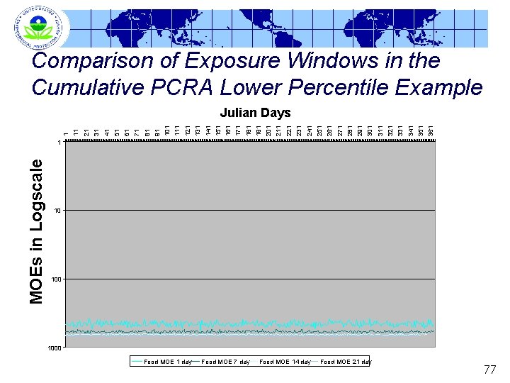
Comparison of MOE Using Different Time-Frames DEEM(FCID)/Calendex™ software has various pre-defined options for duration of time-frame § 7 -, 14 -, 21 -, and 28 -day rolling time-frames • Multi-day averaging process § Increases in time-frame over which averaging performed results in: • Attenuation of variability • Increase in the MOE (decrease in exposure) § Degree to which these changes occur dependent upon selected percentile 75

Comparison of Exposure Windows in the Cumulative PCRA Higher Percentile Example 364 353 342 331 320 309 298 287 276 265 254 243 232 221 210 199 188 177 166 155 144 133 122 111 100 89 78 67 56 45 34 23 12 1 Julian Days MOEs in Logscale at the 99. 9 th Percentile 1 10 1000 Food MOE 1 day Food MOE 7 day Food MOE 14 day Food MOE 21 day 76

Comparison of Exposure Windows in the Cumulative PCRA Lower Percentile Example 361 351 341 331 321 311 301 291 281 271 261 251 231 241 211 221 201 191 181 171 161 151 141 131 111 121 101 91 71 81 61 51 41 31 21 1 11 Julian Days MOEs in Logscale 1 10 1000 Food MOE 1 day Food MOE 7 day Food MOE 14 day Food MOE 21 day 77

Questions for the SAP on Assessment of Food Exposure 78

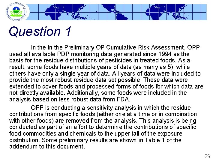
Question 1 In the Preliminary OP Cumulative Risk Assessment, OPP used all available PDP monitoring data generated since 1994 as the basis for the residue distributions of pesticides in treated foods. As a result, some foods have multiple years of data (as many as 5), while others have only a single year of data. All years of data were included to provide the most robust residue data set possible. These data were extended to cover foods and processed forms of foods for which data are not directly available. Additionally, some foods were included in the analysis based on less robust data from FDA. OPP is conducting a sensitivity analysis in which the residue contributions from specific foods (either one at a time or in combination with other foods) are removed from the analysis. This analysis is being conducted as part of an effort to determine the contributions of specific food commodities and chemicals to the upper tail of the exposure distribution. Some preliminary results are shown in Table 1 of the addendum to this document. 79

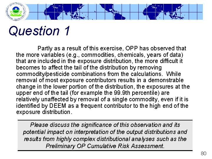
Question 1 Partly as a result of this exercise, OPP has observed that the more variables (e. g. , commodities, chemicals, years of data) that are included in the exposure distribution, the more difficult it becomes to affect the tail of the distribution by removing commodity/pesticide combinations from the calculations. While removal of most exposure contributors results in a demonstrable change in the lower portion of the distribution, the exposures at the upper end of the tail (for example the 99. 9 th percentile) are relatively unaffected by removal of a single commodity, even if it is identified by DEEM as a frequent contributor to the high end of the exposure distribution. Please discuss the significance of this observation and its potential impact on interpretation of the output distributions and results from highly complex distributional analyses such as the Preliminary OP Cumulative Risk Assessment. 80

Question 2 A The Calendex model can be used in a number of modes to develop a profile of exposure estimates. In the current assessment, OPP conducted a series of single-day assessments arrayed chronologically to develop a response surface of exposures. A constant percentile of exposure was selected to represent the potential exposure to a given percentile of the population. For example, the 99 th percentile for each day would be arrayed for 365 days to reflect the population estimate across the calendar year. Calendex can also be used in a multi-day sequential series analysis, also referred to as a “rolling time-frame mode. ” A rolling time-frame provides an estimate of the average of daily exposures for an individual calculated over multiple (7, 14, 21, or 28) days, for each multiple day period over the course of a year, (e. g. , days 1 -7, then days 2 -8, then days 3 -9, etc. ). In this mode, an individual's food exposure is tracked across the calendar year by randomly selecting day one or day two of that individual’s reported consumption from the CSFII and combining each commodity which comprises that consumption with randomly selected residue values for each day of the calendar year. These rolling averages for each individual are assembled to develop a distribution of rolling average exposures. 81

Question 2 A (continued) During previous SAP meetings, the Panel has expressed concern about the use of CSFII records to represent longitudinal consumption patterns for individuals. Concern arose as a result of the design of the CSFII study, in which two nonconsecutive days of data (separated by 3 to 10 days) were collected for each individual. Please comment on the use of CSFII data to support each of these two modes of Calendex as they pertain to the cumulative risk assessment of pesticides in foods. 82

Question 2 B The random selection of PDP residue values assumes that the residues in foods consumed across a series of days are independent of each other. In other words, foods consumed are from unrelated sources and there is no carryover from one day to another. This assumption may be inappropriate given that many consumers obtain food in bulk (i. e. , multiday) quantities that may have similar treatment history and would typically consume this food over a short multi-day period (e. g. , leftovers). In such a case the residues contained in the foods would violate the assumption of independence. Please comment on the use of PDP data to support each of these two modes of Calendex as they pertain to the cumulative risk assessment of pesticides in foods. What issues are likely to accrue from the assumption of independence in residue data? 83

84