Sergios Theodoridis Konstantinos Koutroumbas Version 2 1 PATTERN

Sergios Theodoridis Konstantinos Koutroumbas Version 2 1

PATTERN RECOGNITION v Typical application areas Ø Machine vision Ø Character recognition (OCR) Ø Computer aided diagnosis Ø Speech recognition Ø Face recognition Ø Biometrics Ø Image Data Base retrieval Ø Data mining Ø Bionformatics v The task: Assign unknown objects – patterns – into the correct class. This is known as classification. 2

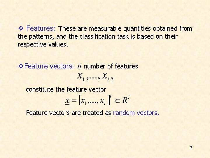
v Features: These are measurable quantities obtained from the patterns, and the classification task is based on their respective values. v. Feature vectors: A number of features constitute the feature vector Feature vectors are treated as random vectors. 3

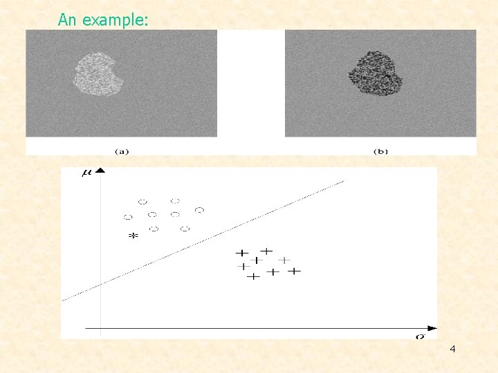
An example: 4

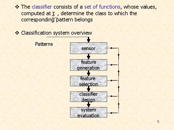
v The classifier consists of a set of functions, whose values, computed at , determine the class to which the corresponding pattern belongs v Classification system overview Patterns sensor feature generation feature selection classifier design system evaluation 5

v Supervised – unsupervised pattern recognition: The two major directions Ø Supervised: Patterns whose class is known a-priori are used for training. Ø Unsupervised: The number of classes is (in general) unknown and no training patterns are available. 6

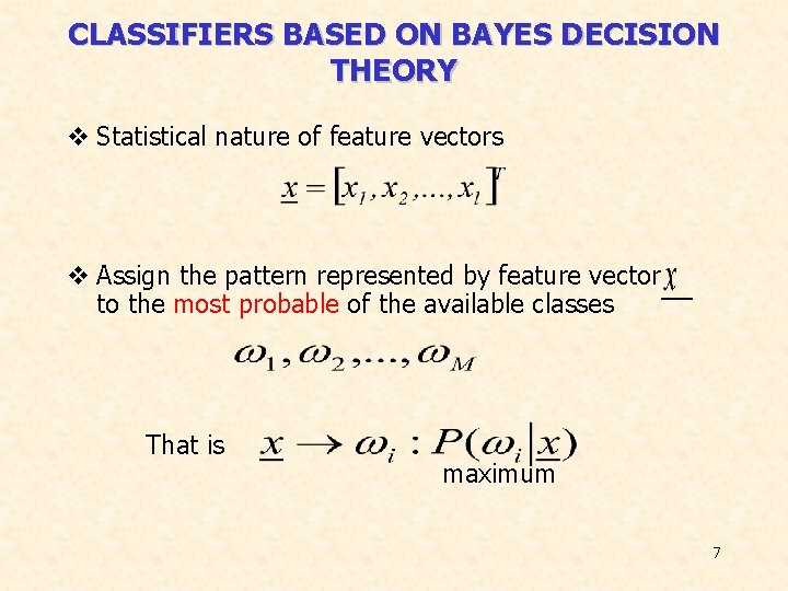
CLASSIFIERS BASED ON BAYES DECISION THEORY v Statistical nature of feature vectors v Assign the pattern represented by feature vector to the most probable of the available classes That is maximum 7

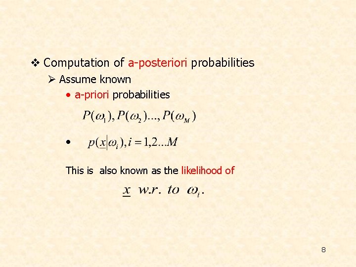
v Computation of a-posteriori probabilities Ø Assume known • a-priori probabilities • This is also known as the likelihood of 8

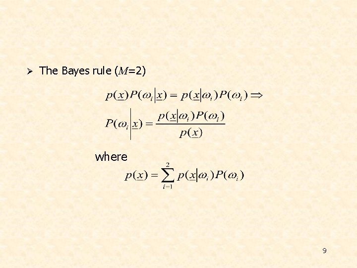
Ø The Bayes rule (Μ=2) where 9

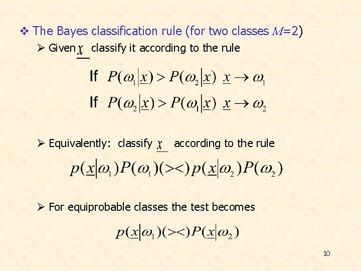
v The Bayes classification rule (for two classes M=2) Ø Given classify it according to the rule Ø Equivalently: classify according to the rule Ø For equiprobable classes the test becomes 10

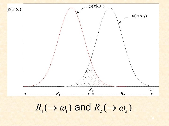
11

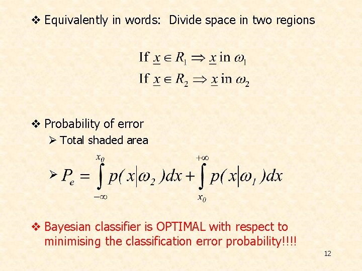
v Equivalently in words: Divide space in two regions v Probability of error Ø Total shaded area Ø v Bayesian classifier is OPTIMAL with respect to minimising the classification error probability!!!! 12

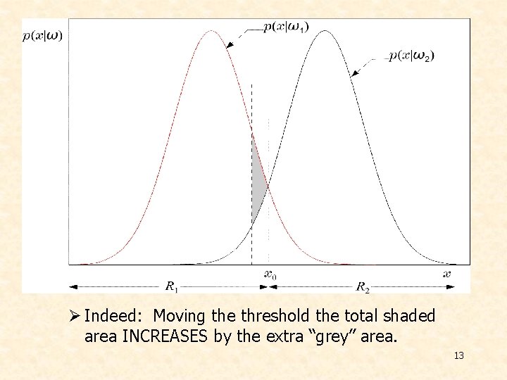
Ø Indeed: Moving the threshold the total shaded area INCREASES by the extra “grey” area. 13

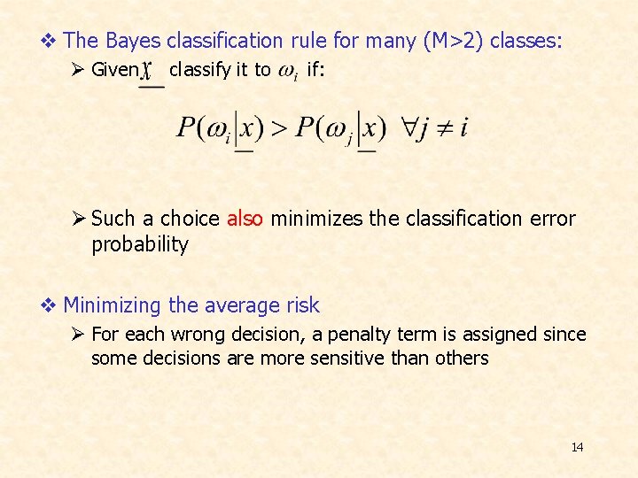
v The Bayes classification rule for many (M>2) classes: Ø Given classify it to if: Ø Such a choice also minimizes the classification error probability v Minimizing the average risk Ø For each wrong decision, a penalty term is assigned since some decisions are more sensitive than others 14

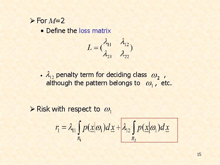
Ø For M=2 • Define the loss matrix • penalty term for deciding class although the pattern belongs to , , etc. Ø Risk with respect to 15

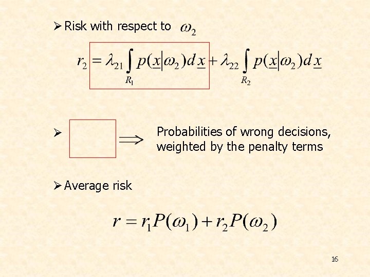
Ø Risk with respect to Ø Probabilities of wrong decisions, weighted by the penalty terms Ø Average risk 16

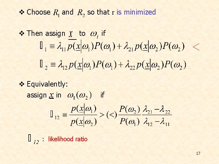
v Choose and v Then assign so that r is minimized to v Equivalently: assign x in if if : likelihood ratio 17

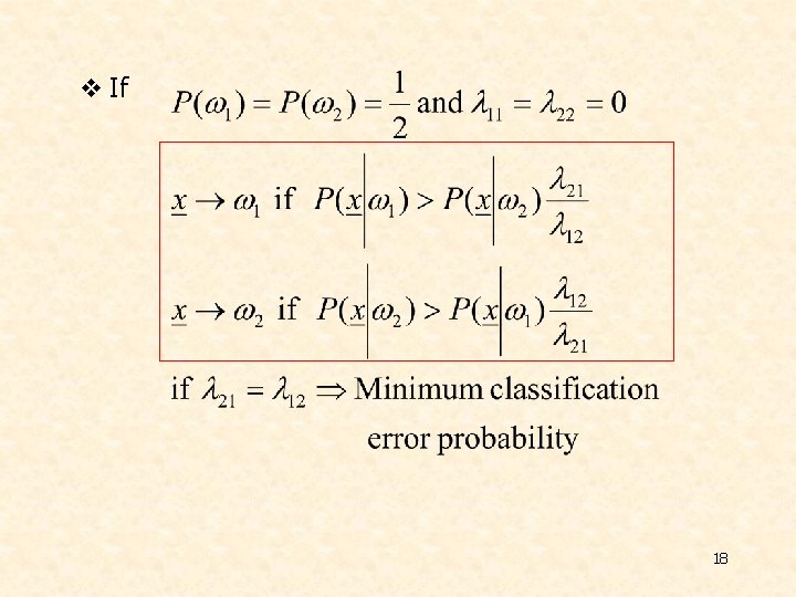
v If 18

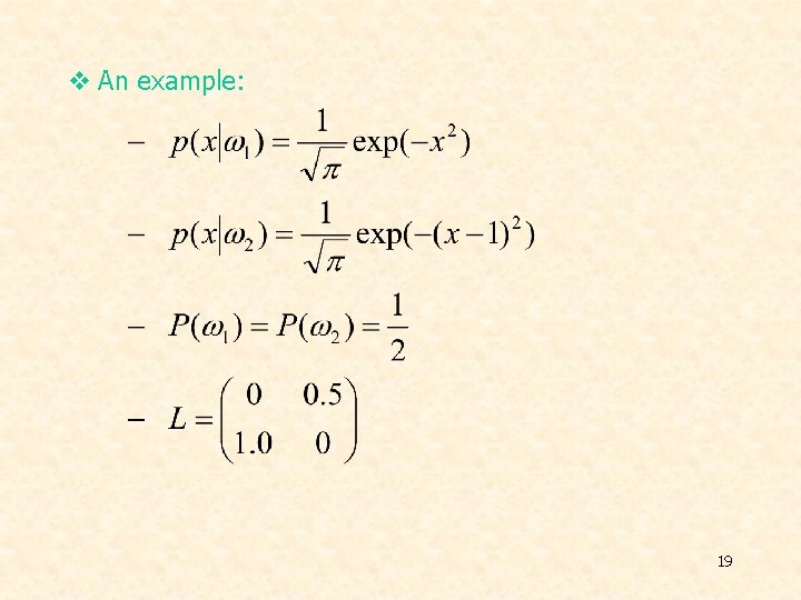
v An example: 19

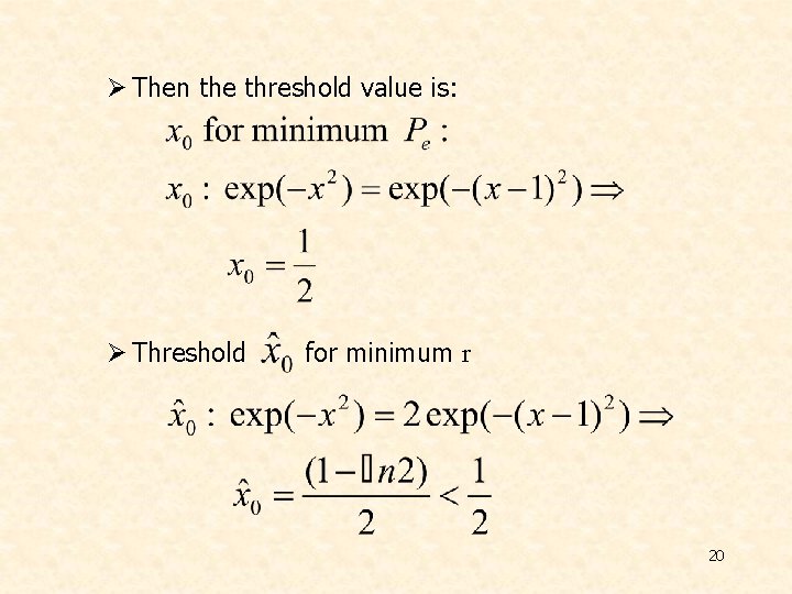
Ø Then the threshold value is: Ø Threshold for minimum r 20

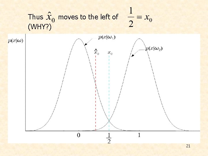
Thus moves to the left of (WHY? ) 21

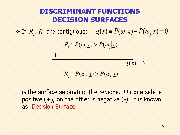
DISCRIMINANT FUNCTIONS DECISION SURFACES v If are contiguous: + - is the surface separating the regions. On one side is positive (+), on the other is negative (-). It is known as Decision Surface 22

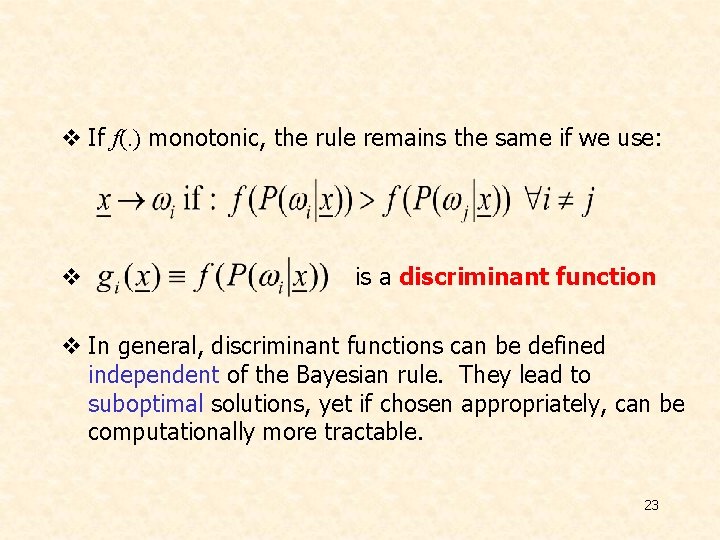
v If f(. ) monotonic, the rule remains the same if we use: v is a discriminant function v In general, discriminant functions can be defined independent of the Bayesian rule. They lead to suboptimal solutions, yet if chosen appropriately, can be computationally more tractable. 23

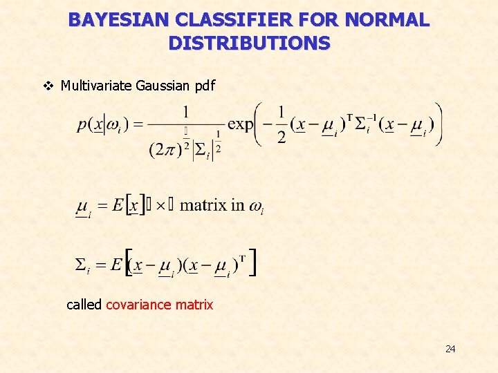
BAYESIAN CLASSIFIER FOR NORMAL DISTRIBUTIONS v Multivariate Gaussian pdf called covariance matrix 24

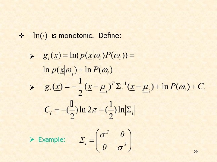
is monotonic. Define: v Ø Ø Ø Example: 25

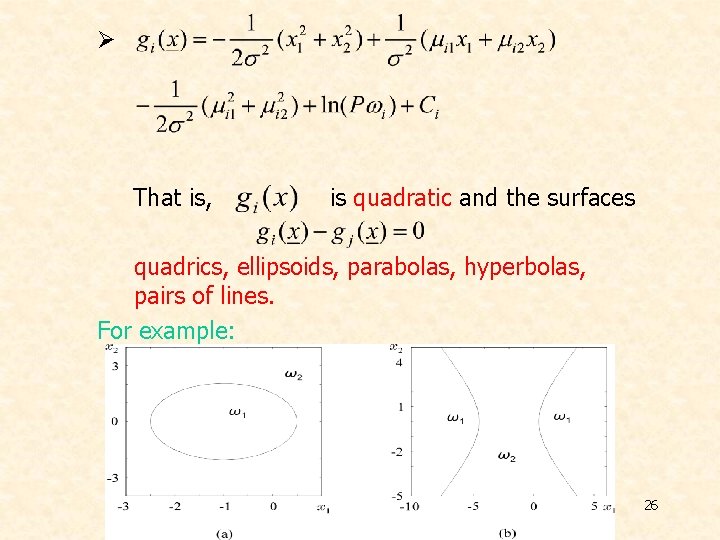
Ø That is, is quadratic and the surfaces quadrics, ellipsoids, parabolas, hyperbolas, pairs of lines. For example: 26

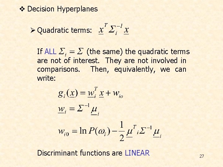
v Decision Hyperplanes Ø Quadratic terms: If ALL (the same) the quadratic terms are not of interest. They are not involved in comparisons. Then, equivalently, we can write: Discriminant functions are LINEAR 27

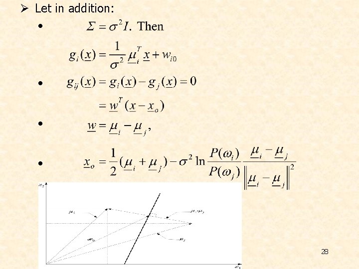
Ø Let in addition: • • 28

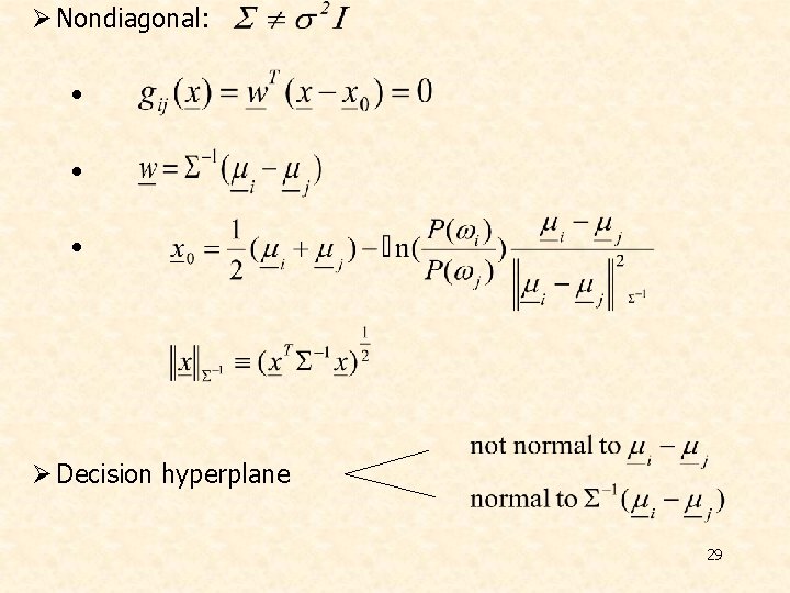
Ø Nondiagonal: • • • Ø Decision hyperplane 29

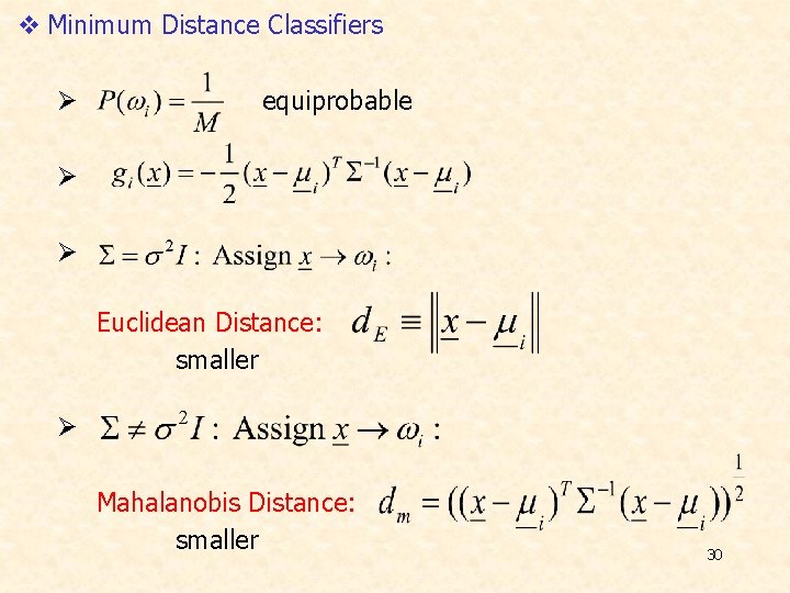
v Minimum Distance Classifiers Ø equiprobable Ø Ø Euclidean Distance: smaller Ø Mahalanobis Distance: smaller 30

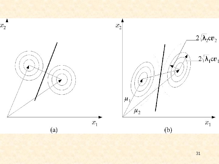
31

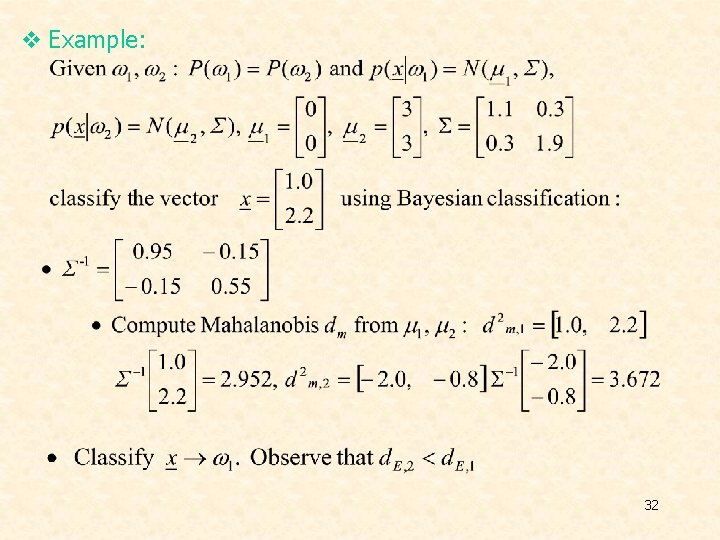
v Example: 32

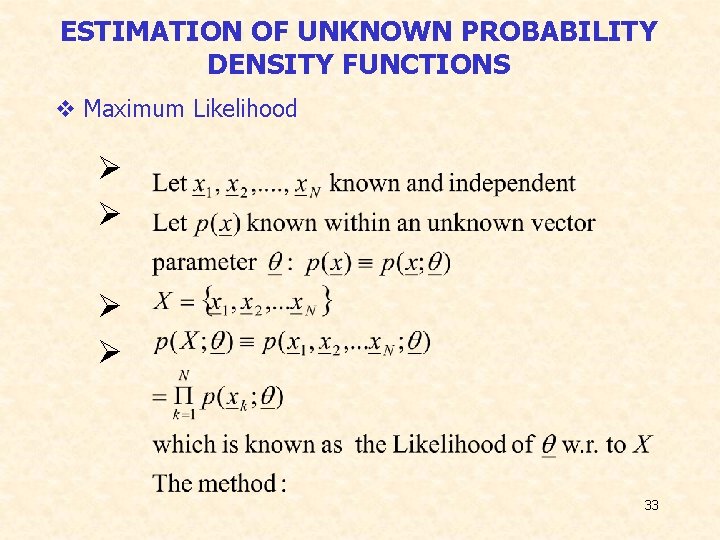
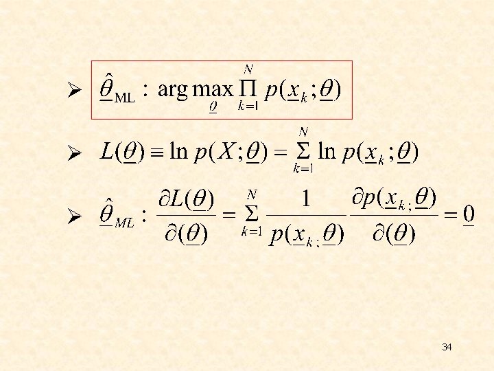
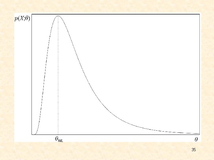
ESTIMATION OF UNKNOWN PROBABILITY DENSITY FUNCTIONS v Maximum Likelihood Ø Ø 33

35

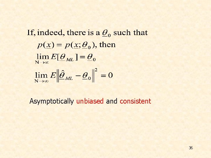
Asymptotically unbiased and consistent 36

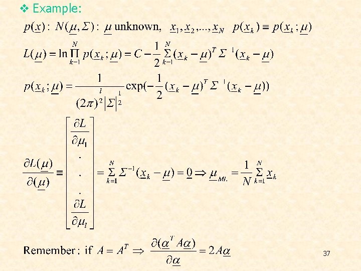
v Example: 37

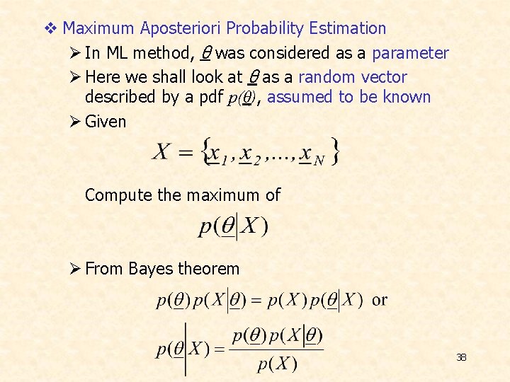
v Maximum Aposteriori Probability Estimation Ø In ML method, θ was considered as a parameter Ø Here we shall look at θ as a random vector described by a pdf p(θ), assumed to be known Ø Given Compute the maximum of Ø From Bayes theorem 38

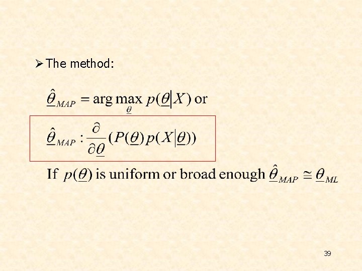
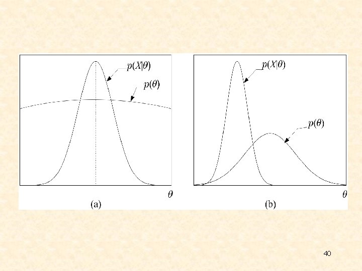
Ø The method: 39

40

v Example: 41

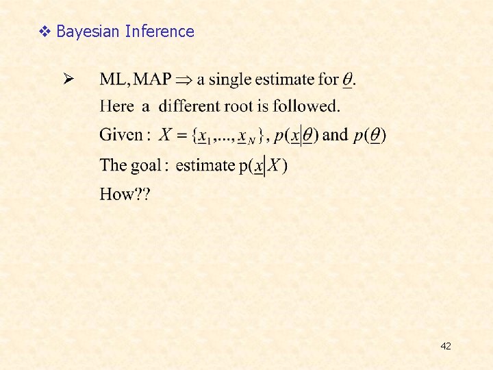
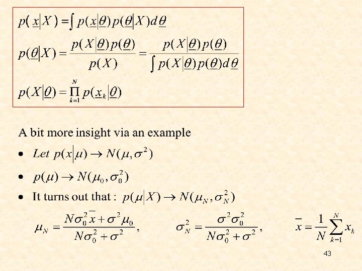
v Bayesian Inference Ø 42

43

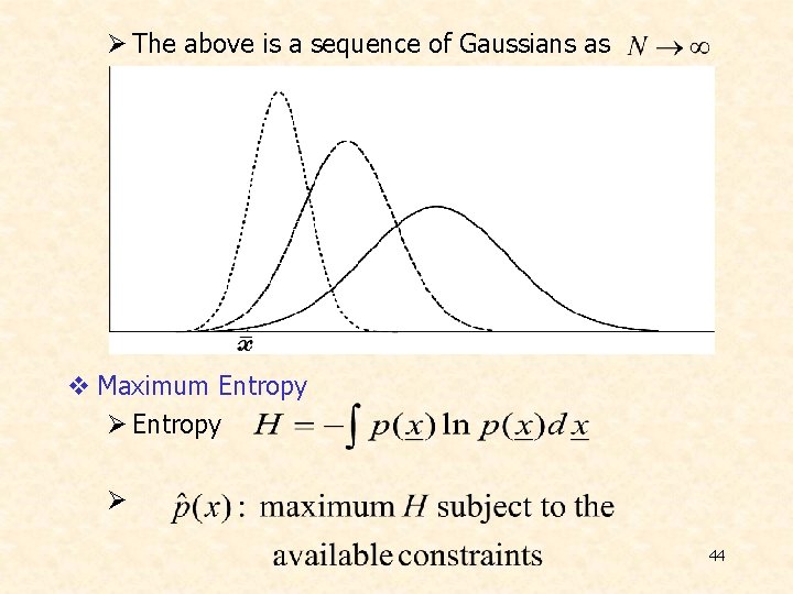
Ø The above is a sequence of Gaussians as v Maximum Entropy Ø 44

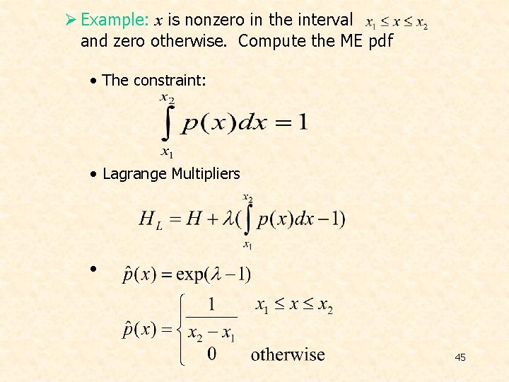
Ø Example: x is nonzero in the interval and zero otherwise. Compute the ME pdf • The constraint: • Lagrange Multipliers • 45

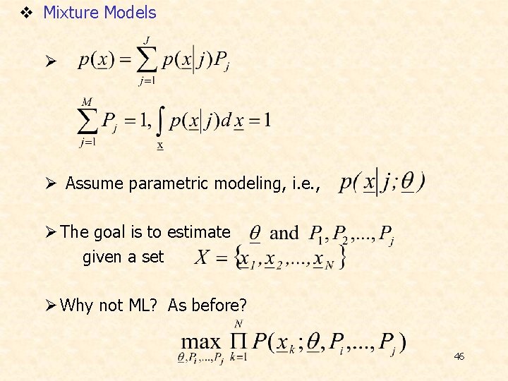
v Mixture Models Ø Ø Assume parametric modeling, i. e. , Ø The goal is to estimate given a set Ø Why not ML? As before? 46

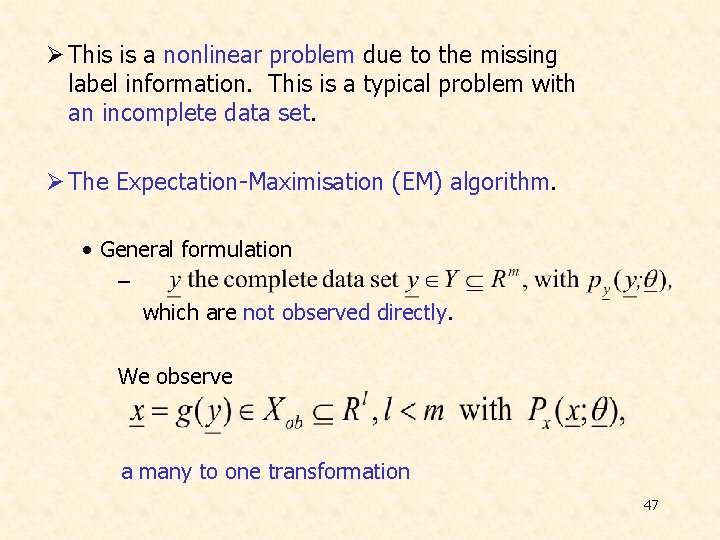
Ø This is a nonlinear problem due to the missing label information. This is a typical problem with an incomplete data set. Ø The Expectation-Maximisation (EM) algorithm. • General formulation – which are not observed directly. We observe a many to one transformation 47

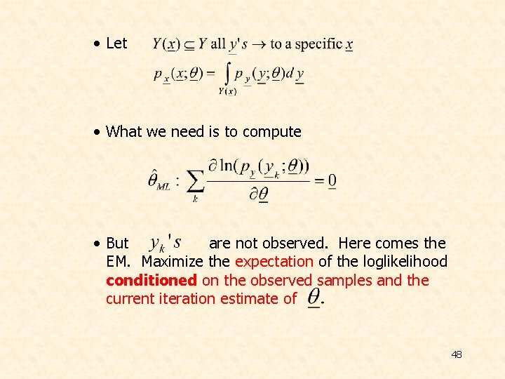
• Let • What we need is to compute • But are not observed. Here comes the EM. Maximize the expectation of the loglikelihood conditioned on the observed samples and the current iteration estimate of 48

Ø The algorithm: • E-step: • M-step: Ø Application to the mixture modeling problem • Complete data • Observed data • • Assuming mutual independence 49

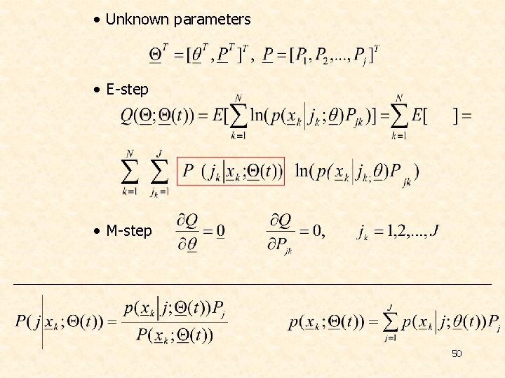
• Unknown parameters • E-step • M-step 50

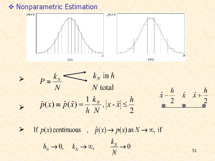
v Nonparametric Estimation Ø Ø Ø 51

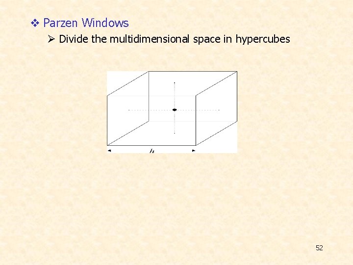
v Parzen Windows Ø Divide the multidimensional space in hypercubes 52

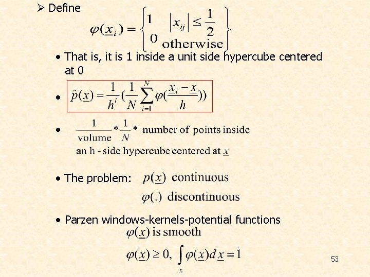
Ø Define • That is, it is 1 inside a unit side hypercube centered at 0 • • • The problem: • Parzen windows-kernels-potential functions 53

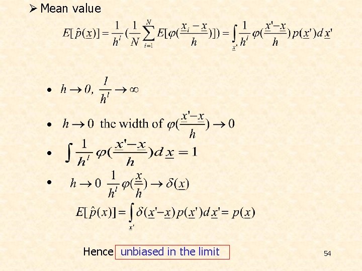
Ø Mean value • • Hence unbiased in the limit 54

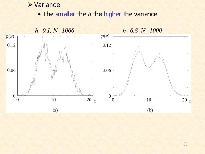
Ø Variance • The smaller the higher the variance h=0. 1, N=1000 h=0. 8, N=1000 55

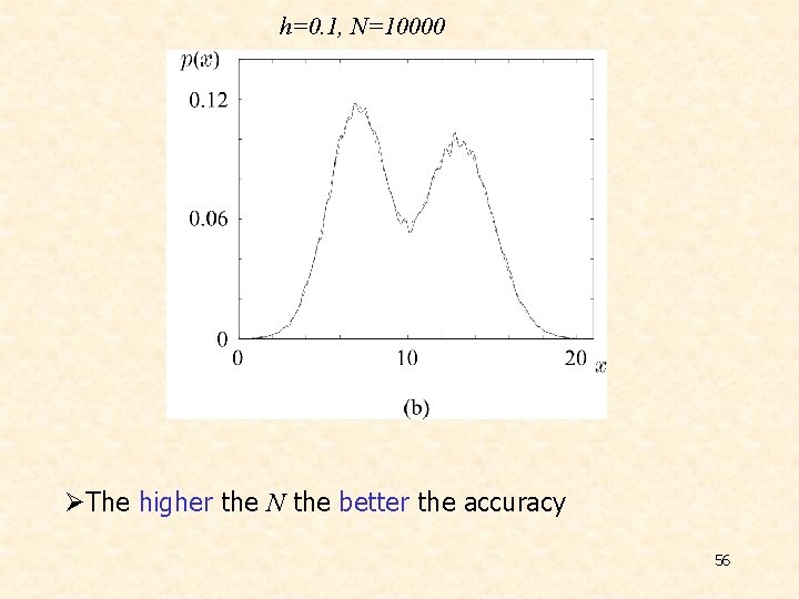
h=0. 1, N=10000 ØThe higher the N the better the accuracy 56

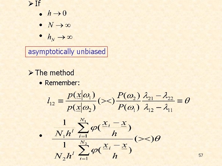
Ø If • • • asymptotically unbiased Ø The method • Remember: • 57

v CURSE OF DIMENSIONALITY Ø In all the methods, so far, we saw that the highest the number of points, N, the better the resulting estimate. Ø If in the one-dimensional space an interval, filled with N points, is adequately (for good estimation), in the two-dimensional space the corresponding square will require N 2 and in the ℓ-dimensional space the ℓdimensional cube will require Nℓ points. Ø The exponential increase in the number of necessary points in known as the curse of dimensionality. This is a major problem one is confronted with in high dimensional spaces. 58

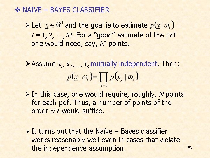
v NAIVE – BAYES CLASSIFIER Ø Let and the goal is to estimate i = 1, 2, …, M. For a “good” estimate of the pdf one would need, say, Nℓ points. Ø Assume x 1, x 2 , …, xℓ mutually independent. Then: Ø In this case, one would require, roughly, N points for each pdf. Thus, a number of points of the order N·ℓ would suffice. Ø It turns out that the Naïve – Bayes classifier works reasonably well even in cases that violate the independence assumption. 59

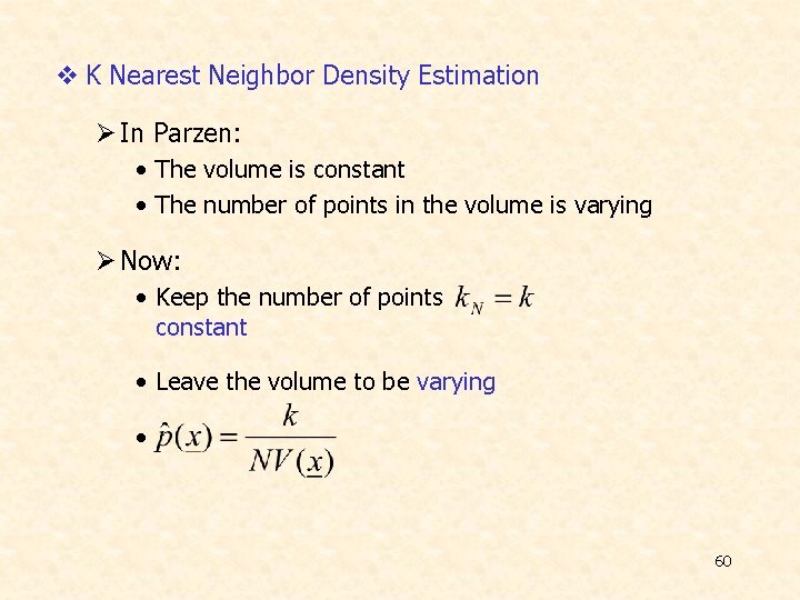
v K Nearest Neighbor Density Estimation Ø In Parzen: • The volume is constant • The number of points in the volume is varying Ø Now: • Keep the number of points constant • Leave the volume to be varying • 60

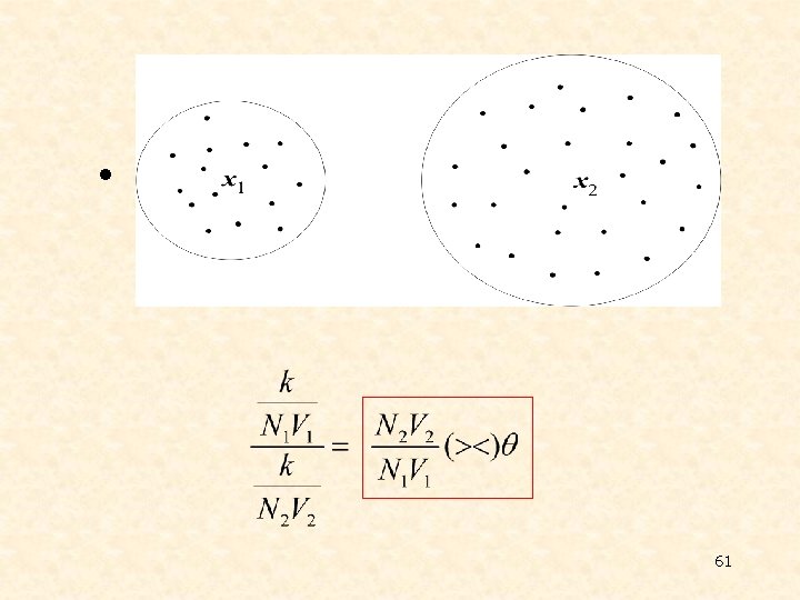
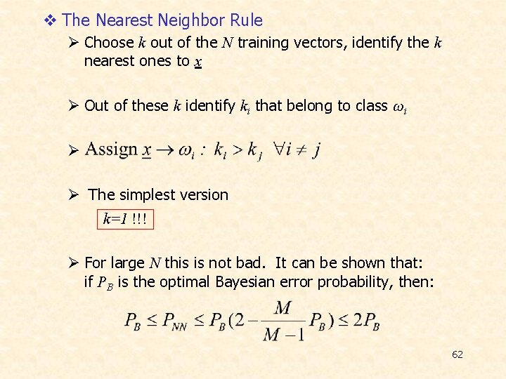
v The Nearest Neighbor Rule Ø Choose k out of the N training vectors, identify the k nearest ones to x Ø Out of these k identify ki that belong to class ωi Ø Ø The simplest version k=1 !!! Ø For large N this is not bad. It can be shown that: if PB is the optimal Bayesian error probability, then: 62

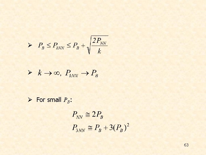
Ø Ø Ø For small PB: 63

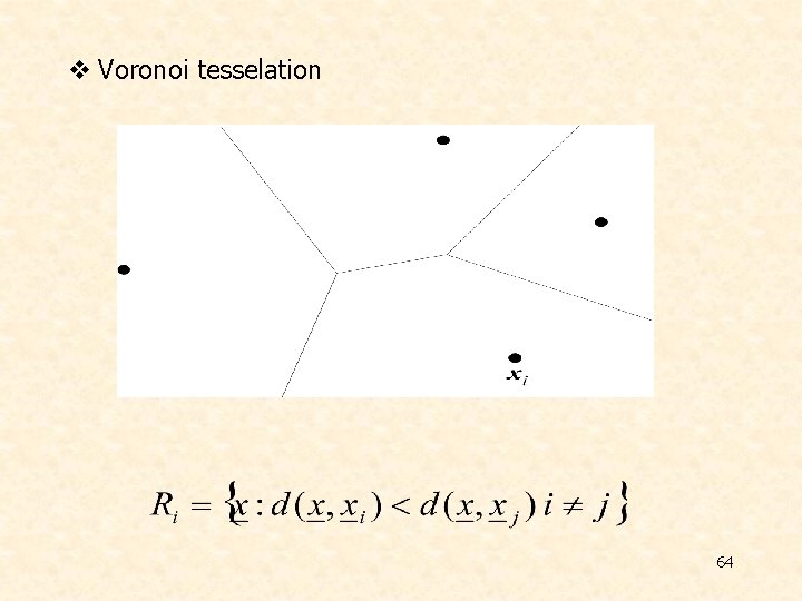
v Voronoi tesselation 64

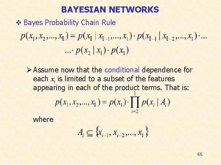
BAYESIAN NETWORKS v Bayes Probability Chain Rule Ø Assume now that the conditional dependence for each xi is limited to a subset of the features appearing in each of the product terms. That is: where 65

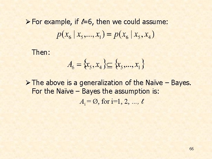
Ø For example, if ℓ=6, then we could assume: Then: Ø The above is a generalization of the Naïve – Bayes. For the Naïve – Bayes the assumption is: Ai = Ø, for i=1, 2, …, ℓ 66

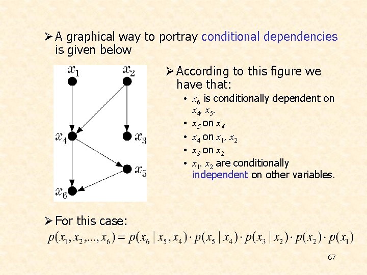
Ø A graphical way to portray conditional dependencies is given below Ø According to this figure we have that: • x 6 is conditionally dependent on x 4 , x 5. • x 5 on x 4 • x 4 on x 1, x 2 • x 3 on x 2 • x 1, x 2 are conditionally independent on other variables. Ø For this case: 67

v Bayesian Networks Ø Definition: A Bayesian Network is a directed acyclic graph (DAG) where the nodes correspond to random variables. Each node is associated with a set of conditional probabilities (densities), p(xi|Ai), where xi is the variable associated with the node and Ai is the set of its parents in the graph. Ø A Bayesian Network is specified by: • The marginal probabilities of its root nodes. • The conditional probabilities of the non-root nodes, given their parents, for ALL possible combinations. 68

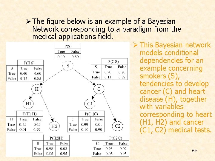
Ø The figure below is an example of a Bayesian Network corresponding to a paradigm from the medical applications field. Ø This Bayesian network models conditional dependencies for an example concerning smokers (S), tendencies to develop cancer (C) and heart disease (H), together with variables corresponding to heart (H 1, H 2) and cancer (C 1, C 2) medical tests. 69

Ø Once a DAG has been constructed, the joint probability can be obtained by multiplying the marginal (root nodes) and the conditional (non-root nodes) probabilities. Ø Training: Once a topology is given, probabilities are estimated via the training data set. There also methods that learn the topology. Ø Probability Inference: This is the most common task that Bayesian networks help us to solve efficiently. Given the values of some of the variables in the graph, known as evidence, the goal is to compute the conditional probabilities for some of the other variables, given the evidence. 70

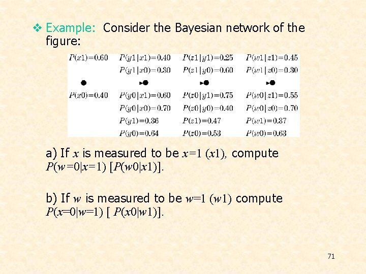
v Example: Consider the Bayesian network of the figure: a) If x is measured to be x=1 (x 1), compute P(w=0|x=1) [P(w 0|x 1)]. b) If w is measured to be w=1 (w 1) compute P(x=0|w=1) [ P(x 0|w 1)]. 71

Ø For a), a set of calculations are required that propagate from node x to node w. It turns out that P(w 0|x 1) = 0. 63. Ø For b), the propagation is reversed in direction. It turns out that P(x 0|w 1) = 0. 4. Ø In general, the required inference information is computed via a combined process of “message passing” among the nodes of the DAG. v Complexity: Ø For singly connected graphs, message passing algorithms amount to a complexity linear in the number of nodes. 72