Sequential variational method for data assimilation without tangent


: 1000")


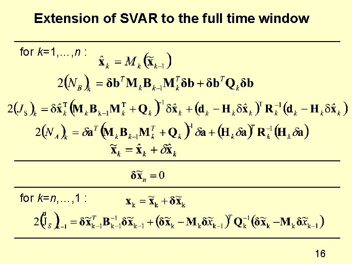


 calculated")


- Slides: 38
Sequential variational method for data assimilation without tangent linear and adjoint model integrations Srdjan Dobricic, CMCC, Bologna, Italy 1
Outline • Weak 4 DVAR formulation • Motivation • Theoretical decomposition • Approximation with TL and adjoint models • Approximation without TL and adjoint models • Computationally efficient solution for backward steps 2
Weak 4 DVAR formulation Weak 4 DVAR with non-linear model and observational operators, assume that the errors are uncorrelated in time. Temporal biases are ignored! Linearization: 3
Motivation • Weak formulation of the 4 DVAR may require the definition of a very large dimension of the parameter state • The 4 DVAR does not provide an estimate of background error covariances at the end of the time window • In comparison to the extended Kalman filter the linearization may be less accurate when the time window is long. • The variational formulation requires the development of a tangent linear model approximation and especially its adjoint 4
Dimension of parameter space for Mediterranean Forecasting System re-analyses Model state size (daily): 1000 x 250 x 100 x 4 = 108 Model state size (pentad): 1000 x 250 x 100 x 4 x 350 x 5= 1011 5
Single time step sequential estimate 4 DVAR with a single time step: Partial derivate with respect to 6
Single time step sequential estimate 7
Single sequential step This also the gradient of the following cost function: 8
Single time step sequential estimate at k-1 Has the minimum for the same like: 9
Temporal evolution of background error covariances How to estimate or ? For example it may be done by directly multiplying matrices, by ensemble methods or by sequential Monte Carlo methods. Here I propose two well known variational algorithms: Lanczos and BFGS. (Lanczos algorithm in fact has a more general application in linear algebra. ) 10
Temporal evolution of background error covariances We may form the following cost function: where Its minimum is know and given by: We can ignore that we know it and iterate the cost function to indirectly estimate the partial eigenvalue decomposition of its second derivative: 11
Temporal evolution of background error covariances The cost function to estimate is: It can be rewritten in the following form: 12
Temporal evolution of background error covariances The sequence of operations with the Lanczos algorithm: 1. Make a random perturbation 2. Propagate it backwards with 3. Weight to get with 4. Propagate forward with 5. The result gives the gradient of the cost function with respect to the initial perturbation 6. Lanczos or BFGS estimates the next perturbation. 7. Go to step 2. 13
Update of background error covariances We may estimate the update of the background error covariances by finding the inverse of the second derivative of the following cost function: In practice the result is different from finding the second derivative of: 14
Lanczos algorithm It iterativelly estimates elements of symmetric tridiagonal matrix T and matrix Q with columns forming orthonormal basis for the Krylov subspaces (Lanczos vectors). Matrices T and Q satisfy: In each iteration of the algorithm a new Lanczos vector is estimated in a way that it is orthogonal to all the previous Lanczos vectors and that it has the largest norm of all Lanczos vectors orthogonal to the previous Lanczos vectors. 15
Nonlinear trajectory SVAR estimates non-linear trajectory by combining the information from the model and all previous observations, just like the extended Kalman filter. 18
Practical forward implementation with TL and adjoint models The highest computational cost is to estimate The predicted matrix is divided on the evolved and the steady parts 19
Forward steps only with non-linear model integrations 20
Arnoldi algorithm It is an extension of the Lanczos algorithm to the case when the square matrix C is not symmetric. It estimates elements of upper Hessenberg matrix HS and matrix SR with on columns forming orthonormal basis for the Krylov subspaces (Ritz vectors). Matrices HS and SR satisfy: In each iteration of the algorithm a new column of SR is estimated in a way that it is orthogonal to all the previous columns and that the eigenvalues of the Hessenberg matrix HS approximate the largest eigenvalues of C. 21
Forward steps only with non-linear model integrations - Upper Hessenberg matrix 22
Forward steps only with non-linear model integrations
Forward steps only with non-linear model integrations 24
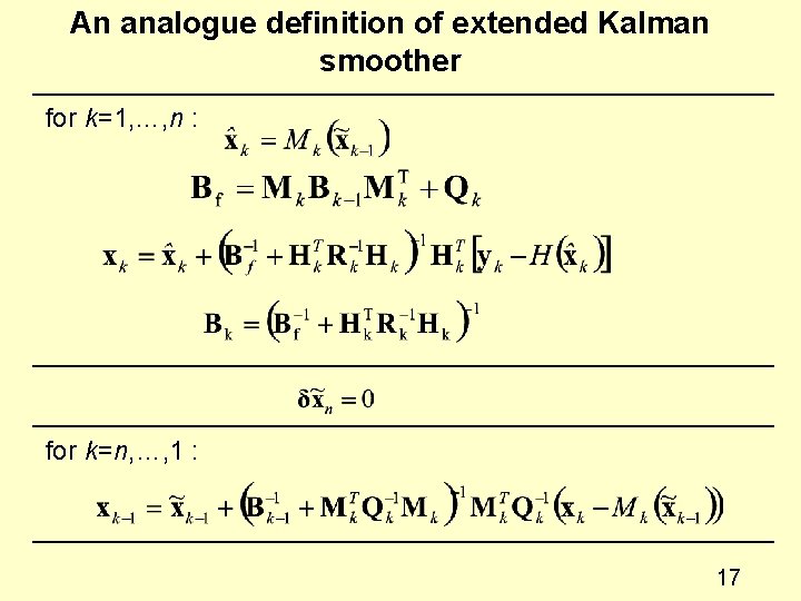
Computationally efficient and numerically stable backward steps SVAR Kalman smoother 25
Computationally efficient and numerically stable backward steps 26
Computationally efficient and numerically stable backward steps 27
Computationally efficient and numerically stable backward steps – perfect model 28
Numerical experiment • Full primitive equations oceanographic model • Coarse resolution of 0. 250 • Dimension: 250 x 100 x 4 x 100 = 108 • Thirty days long assimilation window 29
Numerical experiment: temporal evolution of background error covariances 07 Feb 2005 Standard deviation of temperature errors at 50 m (0 C*102). 07 May 2005 30
Numerical experiment: temporal evolution of background error covariances 50 m covarinces with temperature at point at 30 m depth (values are multiplied by 104). Temperature (C 2) Salinity (C) 07 Feb 2005 07 May 2005
Numerical experiment: temporal evolution of background error covariances Trace of Bk.
Numerical experiment: temporal evolution of background error covariances Trace of Bk.
Numerical experiment: temporal evolution of background error covariances Trace of Bk.
Numerical experiment: backward steps The maximum kinetic energy of surface velocity increments (cm 2 s-2) during backwards steps
Numerical experiment: backward steps The RMS of residuals for the SLA observations (cm) calculated in each assimilation step (dashed line – 3 DVAR, full line – SVAR)
Discussion – relation to predictability • In short term the predictability strongly depends on the initial state and its probability distribution • In longer term an efficient way to estimate the pdf of the solution is to run an ensemble of Gaussian distributions and calculate a weighted sum 37
Conclusions • SVAR splits a large state space problem into several smaller state space problems • It provides an estimate of evolved background error covariances • The non-linear trajectory is estimated like in the extended Kalman filter • In practice the compuational time is made similar to that of 4 DVAR • Each equation of SVAR has an analogue in Kalman smoother equations, but here they are solved variationally • It is possible to solve SVAR without coding tangent-linear and adjoint models 38