Sequential Tests Ph D Course Sequential Tests The

Sequential Tests Ph. D Course

Sequential Tests The question arises that it would not be possible to construct a test that minimizes the sum of first and second type error probabilities? Abraham Wald (1902 -1950) has developed a sequential statistical test that minimizes the expected number of sample elements along with error probabilities. This method is of great importance when sampling is costly because of the destruction of the product under investigation. For example, testing of explosives, bulb life testing, food composition analysis, etc.

Abraham Wald (1902– 1950) – Founder of Sequential Analysis Abraham Wald (Hungarian: Wald Ábrahám), was a mathematician born in Kolozsvár, in then Austria–Hungary (present-day Romania) who contributed to decision theory, geometry, and econometrics, and founded the field of statistical sequential analysis. He spent his researching years at Columbia University.

Sequential testing We have set up the testing problem as if we were forced to take a decision: accept or reject the null hypothesis. But suppose that we in fact rather would say that the matter is not clear and we would wich to collect additional observations. The idea behind the sequential testing is that we collect observations one at a time; when observation Xi = xi has been made, we choose between the following options: • Accept the null hypothesis and stop observation; • Reject the null hypothesis and stop observation; • Defer decision until we have collected another piece of information as Xi+1.

The sequential probability ratio test (SPRT) The challenge is now to find out when to choose which of the above options. We would want to control the two types of error and α = P{Deciding for HA when H 0 is true} probability of type I error b = P{Deciding for H 0 when HA is true} probability of type II error Note that it is traditional in this context to treat HA and H 0 symmetrically.

Recall that the standard LRT has critical region of the form Wald’s Sequential Probability Ratio Test (SPRT) has the following form:

It can be shown that the SPRT is optimal in the sense that it minimizes the average sample size before a decision is made among all sequential tests which do not have larger error probabilities than the SPRT. It can also be shown that the boundaries A and B can be calculated as with very good approximation as so the SPRT is really very simple to apply in practice.

Optimality of SPRT

Optimality of SPRT

Optimality of SPRT

Example Let's assume the lifetime of a component is described by a Weibull distribution with the shape parameter b = 1. 5. We will use SPRT to determine if the component meets the following h reliability requirements: A target reliability of 92% at 200 hours. If the component meets or exceeds the target reliability, the chance of rejecting it (i. e. , Type I error or α error) should be less than 0. 05. This is comparable to α 2. A minimum reliability of 82% at 200 hours. If the component’s reliability is 82% or less, the probability of accepting it (i. e. , Type II error or β error) should be less than 0. 1. This is comparable to α 1. Our objectives are to: • Calculate the acceptance and rejection line for the SPRT test. • Determine whether to accept or reject the component based on a series of observed failure times.

Solution Using Manual Calculations

T Acceptance Value Rejection Value Decision ID Ti 1 629 15, 775. 24 76, 651. 04125 0 Continue 2 369 22, 863. 5 97, 964. 88014 0 Continue 3 685 40, 791. 66 119, 278. 719 0 Continue 4 270 45, 228. 22 140, 592. 5579 14, 209. 44008 Continue 5 682 63, 038. 74 161, 906. 3968 35, 523. 27897 Continue 6 194 65, 740. 84 183, 220. 2357 56, 837. 11786 Continue 7 113 66, 942. 05 204, 534. 0746 78, 150. 95675 Reject

The plot of the data

EXACT TESTS The exact tests enables us to analyze rare occurrences in large databases or work more accurately with small samples. If we have a small number of case variables with a high percentage of responses in one category, or have to subset your data into fine breakdowns, traditional tests could be incorrect. Exact tests can be useful in situations where the asymptotic assumptions are not met and the asymptotic p-values are not close approximations for the true p-values. Standard asymptotic methods involve the assumption that the test statistic follows a particular distribution when the sample size is sufficiently large. When the sample size is not large, asymptotic results may not be valid, with the asymptotic p-values differing perhaps substantially from the exact p-values. Asymptotic results may also be unreliable when the distribution of the data is sparse, skewed, or heavily tied.

Comparison of tests

Mathematics of a Lady Tasting Tea Ø Given a cup of tea with milk, a lady claims she can discriminate as to whether milk or tea was first added to the cup. Ø To test her claim, eight cups of tea are prepared, four of which have the milk added first and four of which have the tea added first. Ø Question: How many cups does she have to correctly identify to convince us of her ability?

Mathematics of a Lady Tasting Tea The lady in question claimed to be able to tell whether the tea or the milk was added first to a cup. Fisher (one of the quests) proposed to give her eight cups, four of each variety, in random order. Four cups had milk poured first and four cups had tea poured first. The data is known as the Lady Tasting Tea.

H 0: The way of mixing the tea and the lady's ability to recognize are independent of each other H 1: The lady can correctly figure out the order of mixing A lot of times Pearson’s Chi square test is used for this type of analysis but when the assumptions for sample size and cell counts are not met then that approach is not acceptable.

Decision with Pearson Chi square test Although the test accepts the null hypothesis, but the sample size is too small for the application.

Sir Ronald Aylmer Fisher (1890. 02. 17. -1962. 07. 29. ) R. A Fisher proposed an alternative test to the problem. Fisher’s Exact Tests uses the hypergeometric distribution and does not rely on approximations.

Fisher's Exact Test Why use Fisher's Exact Test? • Chi-squared test is suitable only when all the cell frequencies are above a lower bound. • Exact vs. approximate probability distributions.

The derivation

Fisher showed that the probability of obtaining any such set of values was given by the hypergeometric distribution:

Now return to the tea tasting problem! Apply the Fisher method to the given contingency table:

The significance level of the Fisher Independence Exact Test (ie the first type error of the test) is the sum of the probabilities calculated with the hypergeometric formula at which the cellular frequency is at least as favorable to the alternative hypothesis as the one actually observed. This is now 0. 243. (The details later…) We have got that the null hypothesis was much more significant than we did with the Pearson Chi-square test! The test to taste tea does not convince us of the lady's assertion!

Choosing subsets Ø There are 8 × 7 × 6 × 5 = 1680 ways to choose a first cup, a second cup, a third cup, and a fourth cup, in order. Ø There are 4 × 3 × 2 × 1 = 24 ways to order four cups. Ø So the number of ways to choose 4 cups out of 8 is 1680/24 = 70. Ø Note: the lady performs the experiment by selecting 4 cups, say, the ones she claims to have had the tea poured first. Ø For example, the probability that she would correctly identify all 4 cups is 1/70.

Choosing 3 Ø To get exactly 3 right, and, hence, 1 wrong, she would first have to choose 3 from the 4 correct ones. Ø She can do this 4 × 3 × 2 = 24 ways with order. Ø Since 3 cups can be ordered in 3 × 2 = 6 ways, there are 4 ways for her to choose the 3 correctly. Ø Since she can now choose the 1 incorrect cup 4 ways, there a total of 4 × 4 = 16 ways for her to choose exactly 3 right and 1 wrong. Ø Hence the probability that she chooses exactly 3 correctly is 16/70 =8/35.

Statistical significance Ø Suppose the lady correctly identifies all 4 cups. The probability of this when she choose random is 1/70=0. 014. Ø Conclusion § Either she has no ability, and has chosen the correct 4 cups purely by chance, or § she has the discriminatory ability she claims. Ø Since choosing correctly is highly unlikely in the first case (one chance in seventy), we decide for the second. Ø Note: if she got 3 correct and 1 wrong, this would be evidence for her ability, but not persuasive evidence since the chance of getting 3 or more correct is 17/70 = 0. 2429. Ø Note: typically, a result is considered statistically significant if the probability of its occurrence is less than 0. 05, that is, less than 1 out of 20.

Potential values of are 0, 1, 2, 3, 4 , so theoritically the next 2 x 2 contingency tables are possible: Hypergeometrical probability significance level

What would it have been if the lady had recognized the mixtures with same efficiency at a double or triple sample sizes?

Original frequencies n=8, =0, 242 It can be seen that after drinking 24 cup of tea she would have been convincing! Double frequencies n=16, =0, 066 Triple frequencies n=24, =0, 020 33

The Biominal Test Who is going to win an election? Do observed hiring rates of minorities reflect their representation in the population? These questions relate to claims about a binomial proportion p. For example, in an election between two candidates, if p is the probability of candidate A winning, p being greater than or less than. 5 corresponds to candidate A winning or losing, respectively. Generally, we are interested in the hypotheses versus where p is the probability of a success.

The Biominal Test

The Biominal Test What can we do when the sample size small? What is the exact version of the binomial test?

The Biominal Test For quality control, it is examined whether the reject rate produced during manufacture does not exceed the prescribed p 0 = 0. 05 level. In a sample of N = 10 k 0 = 3 rejectamentas were found. How to decide?

In the sample N = 10, the number of rejetamentas follows B (N, p) binomial distribution, where p is the actual rejectamenta ratio in the total population. In the case of a null hypothesis, the probability that the number of rejectamentas is 3 or more:

If we accept the null hypothesis, then the first type of error, with the significance level being maximum (p = p 0 = 0. 05), is 0. 01504: So on = 0. 05 significance level, we reject the null hypothesis!

Executing with IBM SPSS

The run tests

Introduction Let consider a dichotomous sequence which consists of only two elements. Any consecutive subsection consisting same elements in the dichotomous sequence is a run. For example in a coin tossing Bernoulli experiment the symbols T (tail) and H (head) forms a dichotomous sequence. Any consecutive T subsequence or consecutive H subsequence mean a run in the sequence. For example in the sequence TTHTHHHTTHTT we have the next runs: {TT}, {H}, {T}, {HHH}, {TT}, {H}, {TT}. That is this coin tossing sequence consists of 9 runs. The length of the sequence is 18, the number of the 1 length run is 3 ({H}, {T}, {H}), the number of the 2 length run is 4 ({TT}, {TT}), the number of the 3 length run is 1 ({HHH}), and the number of the 4 length run is 1 ({HHHH}).

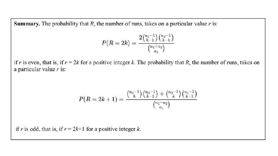
Notations n is the total length of the dichotomous sequence n₁ is the number of the first elements in the sequence n₂ is the number of the second elements in the sequence n=n₁+n₂ Suppose that any permutation of the elements may occur with equal chance. R is the number of the runs in the sequence R is a discrete random variable with range {1, 2, . . . , n}

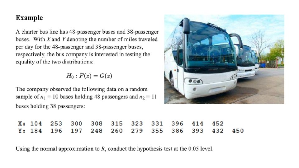
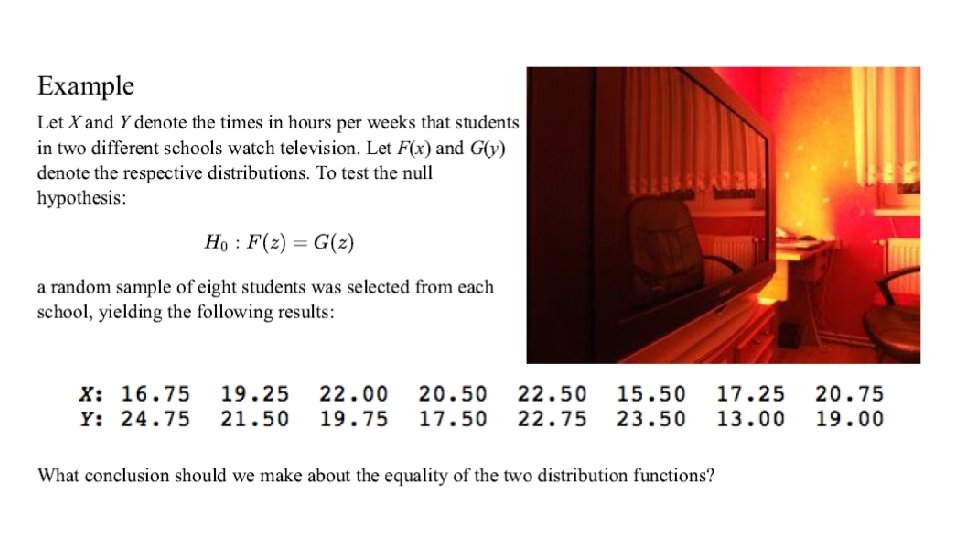
Testing the homogeneity with run test (Wald-Wolfowitz test) We have two independent statistical samples: and

Let's start with the case in which the distributions are equal. In that case, we might observe something like this. The picture suggests that when the distrubutions are equal, the number of runs will likely be large.

An extreme case of the possibilities, when one of the distribution functions is at least great as the other distribution function at all points z. This situation might look something like this: This kind of situation suggests, that when one of the distribution functions is at least as great as the other distribution function the number of runs will likely be small.

Here's another way in which the distribution functions could be unequal: In this case, the medians of X and Y are nearly equal, but the variance of Y is much greater than the variance of X. Again, we would expect the number of runs to be small.

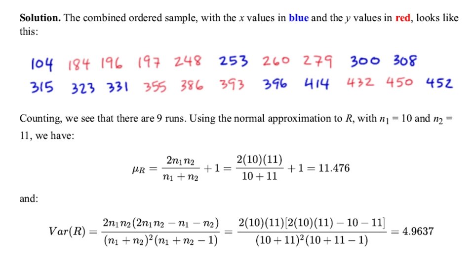
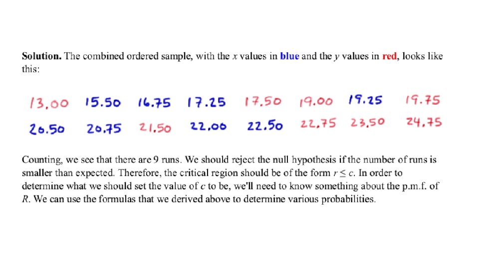
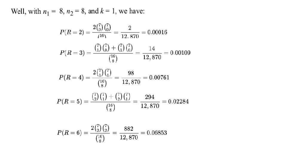
Testing the homogeneity with run test Ø Merge the samples and order the merged sample Ø We consider this ordered sample as a special dichotomous sequence. The elements of the X sample means the first symbol, the elements of the Y sample means the other symbol in the ordered sequence. Ø After this we count the number of the runs: R Ø If the null hypothesis true, R follows the normal distribution with and

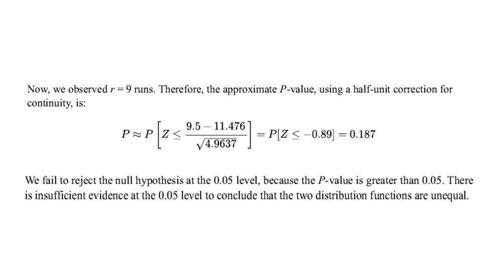
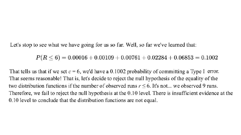
That is, when the null hypothesis is true, ie the two samples have same pdf Decision: we reject the null hypothesis if where

Ø Merge the samples and order the merged sample Ø We consider this ordered sample as a special dichotomous sequence. The elements of the X sample means the first symbol, the elements of the Y sample means the other symbol in the ordered sequence. Ø After this we count the number of the runs: R Decision: we reject the null hypothesis if where

Runs Test for Detecting Non-randomness (Bradley test) The runs test can be used to decide if a data set is from a random process. A run is defined as a series of increasing values or a series of decreasing values. The number of increasing, or decreasing, values is the length of the run. H 0 : H a: the sequence was produced in a random manner the sequence was not produced in a random manner The test statistic is

Runs Test for Detecting Non-randomness

Median test for two samples To test whether or not two samples come from same population, median test is used. It is more efficient than the Wald-Wolfowitz test, but each sample should be size 10 at least. In this case, the hypothesis to be tested is H 0: Two samples come from populations having same distribution. H 1: Two samples come from populations having different distribution. Test Statistic: Chi-square. To test the value of test statistics two samples of sizes n 1 and n 2 combined. Median M of the combined sample size of n=n 1+n 2 is obtained. Number of observations below and above the median M for each sample is determined. This is then analyzedas a 2× 2 contingency table.

Median test for two samples The contingency table to the median test is

Median test for k samples

Median test for k samples

Example: A private bank is interested in finding out whether the customers belonging to two groups differ in their satisfaction level. The two groups are customers belonging to current account holders and savings account holders. A random sample of 20 customers of each category was interviewed regarding their perceptions of the bank's service quality using a Likert-type (ordinal scale) statements. A score of "1" represents very dissatisfied and a score of "5" represents very satisfied. The compiled aggregate scores for each respondent in each group are tabulated be given: What are your conclusions regarding the satisfaction level of these two groups?

Table showing descending order of aggregate score and rank in the combined sample

Grand median is the average of 20 th and 21 st observation = (62+61)/2 =61. 5. Please note that in the above table, average rank is taken whenever the scores are tied. The next step is to prepare a contingency table of two rows and two columns. The cells represent the number of observations that are above and below the grand median in each group. Whenever some observations in each group coincide with the median value, the accepted practice is to first count the observations that are strictly above grand median and put the rest under below grand median. In other words, below grand median in such cases would include less than or equal to grand median.

The calculated test statistic is Critical chi-square for 1 degree of fredom at 5% level of significance is 3. 84. Since the computed chi-square(0. 90) is less than critical chi-square(3. 84), we have no convincing evidence to reject the null hypothesis. Thus the data are consistent with the null hypothesis that there is no difference between the current account holders and savings account holders in the perceived satisfaction level.

The Sign Test The sign test is a non-parametric test which makes very few assumptions about the nature of the distributions under test – this means that it has very general applicability but may lack the statistical power of the alternative tests. The two conditions for the paired-sample sign test are that a sample must be randomly selected from each population, and the samples must be dependent, or paired. Independent samples cannot be meaningfully paired. Since the test is nonparametric, the samples need not come from normally distributed populations. Also, the test works for left-tailed, right-tailed, and two-tailed tests. If X and Y are quantitative variables, the sign test can be used to test the hypothesis that the difference between the X and Y has zero median, assuming continuous distributions of the two random variables X and Y, in the situation when we can draw paired samples from X and Y.

We have a paired sample with n elements: (X 1, Y 1), (X 2, Y 2), …, (Xn, Yn) Assumptions: Let Zi = Yi – Xi for i = 1, . . . , n. 1. The differences Zi are assumed to be independent. 2. Each Zi comes from the same continuous population. 3. The values Xi and Yi represent are ordered (at least the ordinal scale), so the comparisons "greater than", "less than", and "equal to" are meaningful.

The Sign Test To test the null hypothesis, independent pairs of sample data are collected from the populations {(x 1, y 1), (x 2, y 2), . . . , (xn, yn)}. Pairs are omitted for which there is no difference so that there is a possibility of a reduced sample of m pairs. Let p = P(X > Y), and then test the null hypothesis H 0: p = 0. 50. In other words, the null hypothesis states that given a random pair of measurements (xi, yi), then xi and yi are equally likely to be larger than the other. Then let W be the number of pairs for which yi − xi > 0. Assuming that H 0 is true, then W follows a binomial distribution W ~ B(m, 0. 5).

The Sign Test We accept the null hypothesis of the same distribution, if large enough.