Sequential Monte Carlo and Particle Filtering Frank Wood

Sequential Monte Carlo and Particle Filtering Frank Wood Gatsby, November 2007

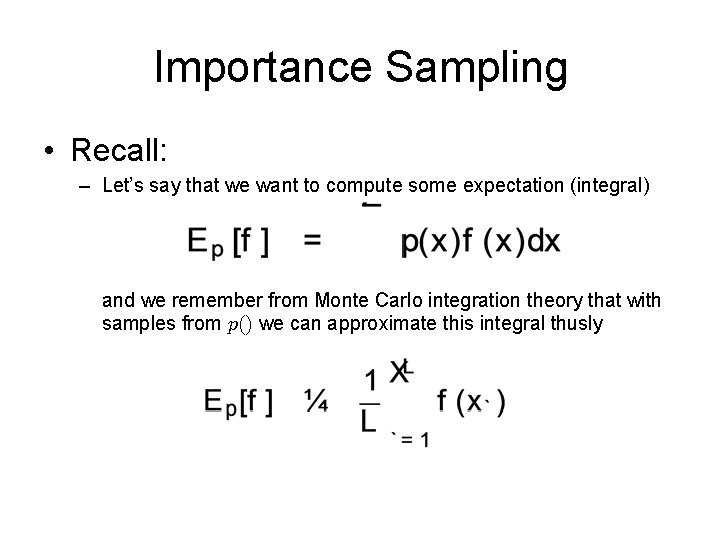
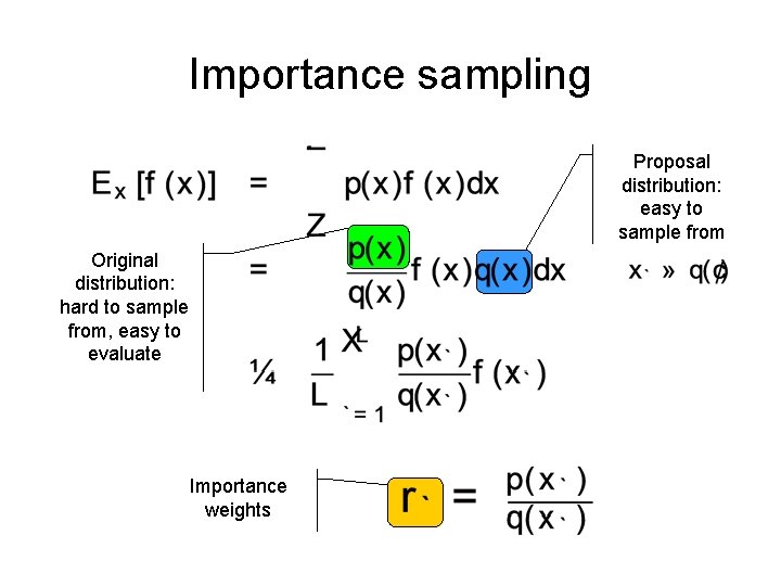
Importance Sampling • Recall: – Let’s say that we want to compute some expectation (integral) and we remember from Monte Carlo integration theory that with samples from p() we can approximate this integral thusly

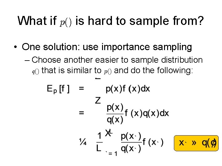
What if p() is hard to sample from? • One solution: use importance sampling – Choose another easier to sample distribution q() that is similar to p() and do the following:

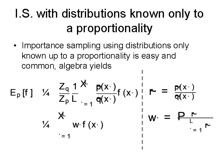
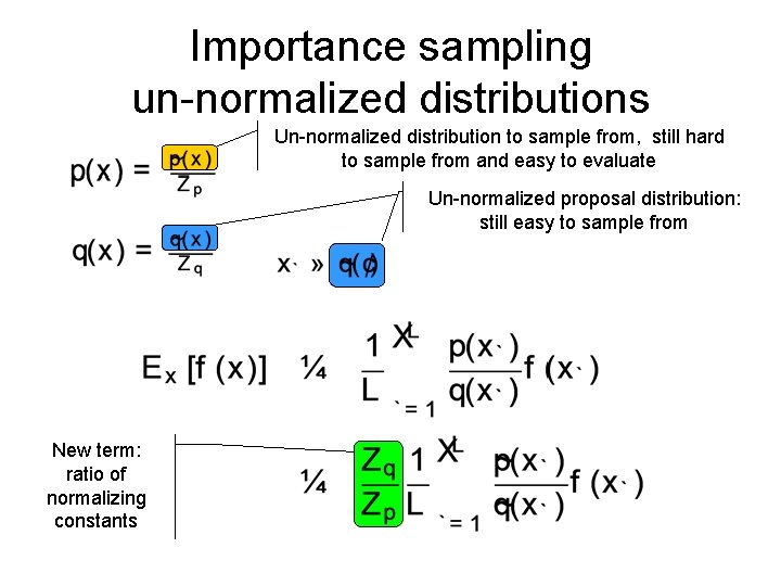
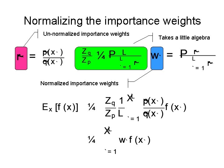
I. S. with distributions known only to a proportionality • Importance sampling using distributions only known up to a proportionality is easy and common, algebra yields

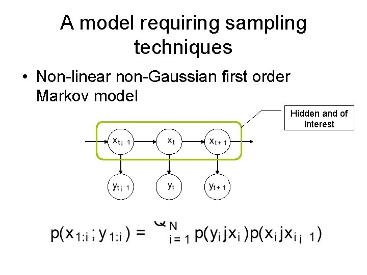
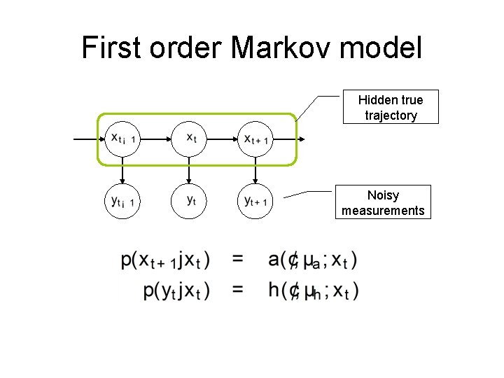
A model requiring sampling techniques • Non-linear non-Gaussian first order Markov model Hidden and of interest \

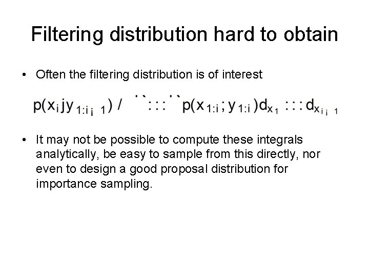
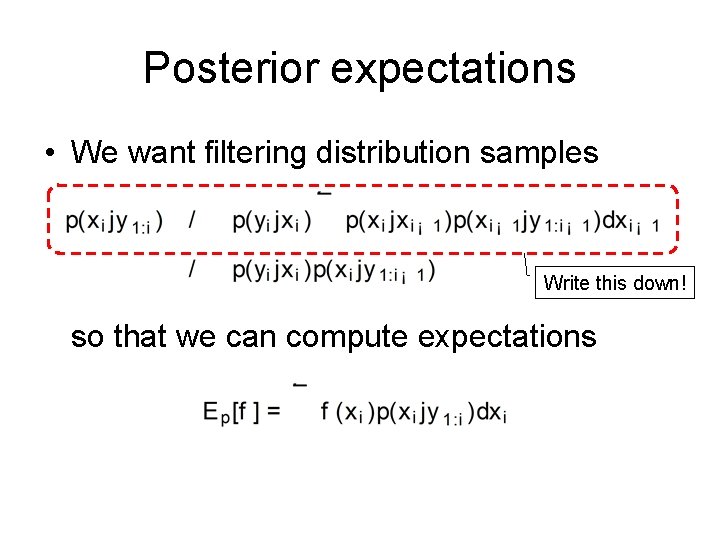
Filtering distribution hard to obtain • Often the filtering distribution is of interest • It may not be possible to compute these integrals analytically, be easy to sample from this directly, nor even to design a good proposal distribution for importance sampling.

A solution: sequential Monte Carlo • Sample from sequence of distributions that “converge” to the distribution of interest • This is a very general technique that can be applied to a very large number of models and in a wide variety of settings. • Today: particle filtering for a first order Markov model

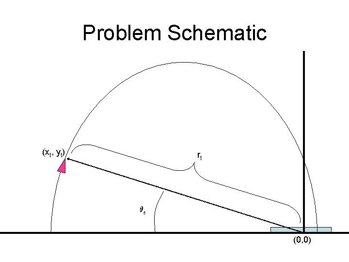
Concrete example: target tracking • A ballistic projectile has been launched in our direction. • We have orders to intercept the projectile with a missile and thus need to infer the projectiles current position given noisy measurements.

Problem Schematic (xt, yt) rt µt (0, 0)

Probabilistic approach • Treat true trajectory as a sequence of latent random variables • Specify a model and do inference to recover the position of the projectile at time t

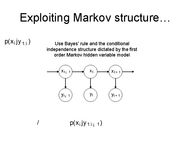
First order Markov model Hidden true trajectory Noisy measurements

Posterior expectations • We want filtering distribution samples Write this down! so that we can compute expectations

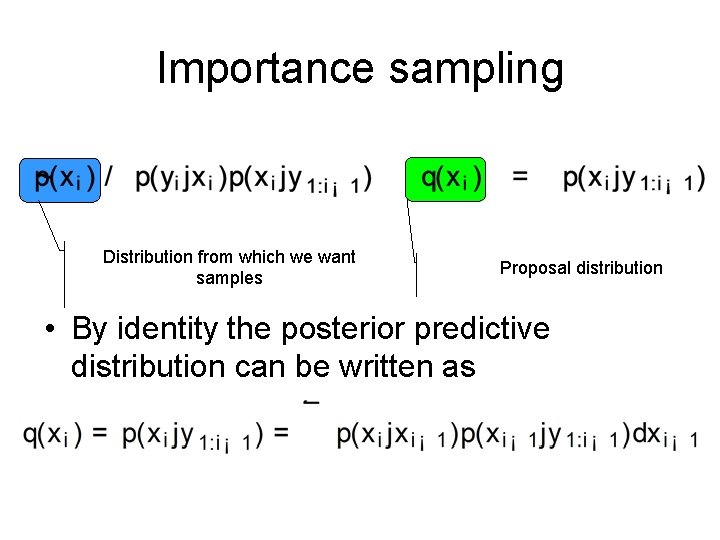
Importance sampling Distribution from which we want samples Proposal distribution • By identity the posterior predictive distribution can be written as

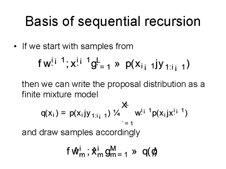
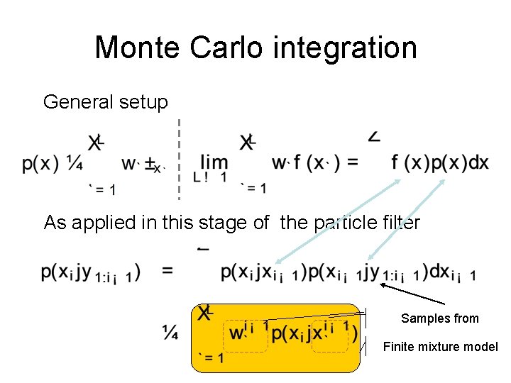
Basis of sequential recursion • If we start with samples from then we can write the proposal distribution as a finite mixture model and draw samples accordingly

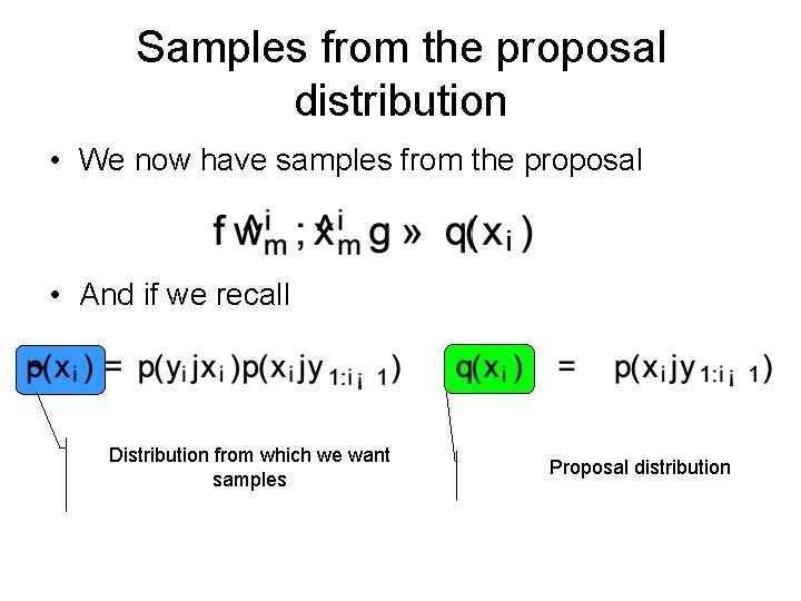
Samples from the proposal distribution • We now have samples from the proposal • And if we recall Distribution from which we want samples Proposal distribution

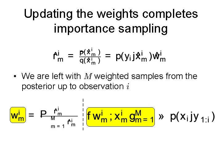
Updating the weights completes importance sampling • We are left with M weighted samples from the posterior up to observation i

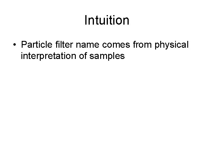
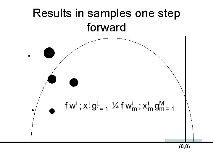
Intuition • Particle filter name comes from physical interpretation of samples

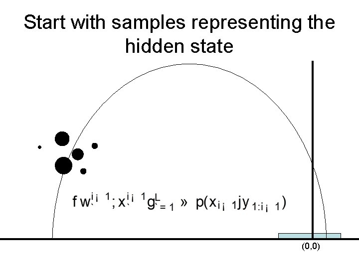
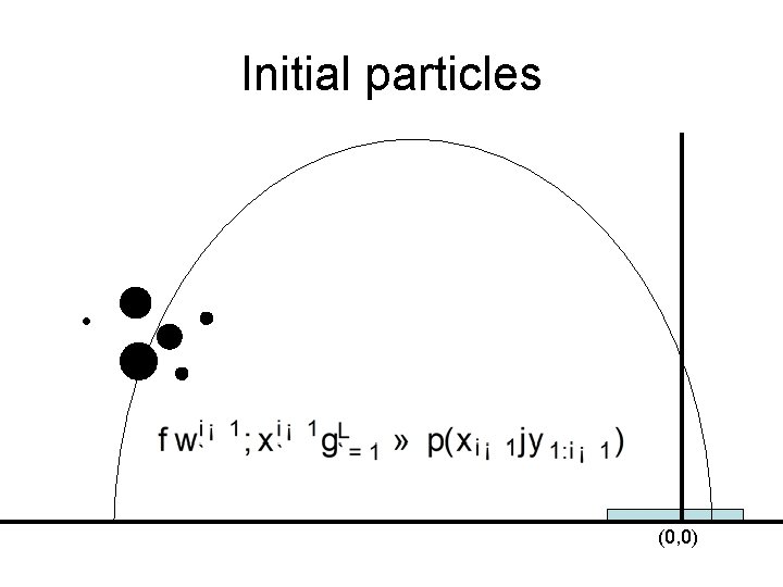
Start with samples representing the hidden state (0, 0)

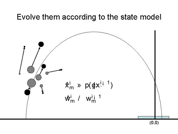
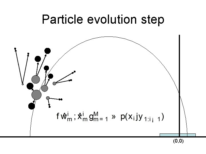
Evolve them according to the state model (0, 0)

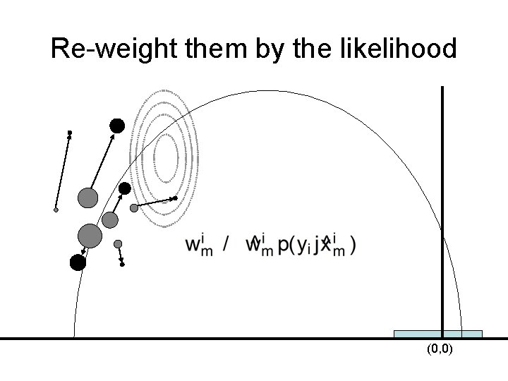
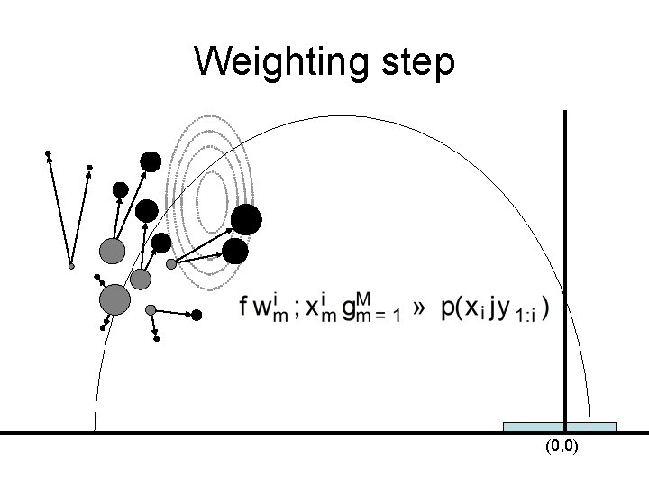
Re-weight them by the likelihood (0, 0)

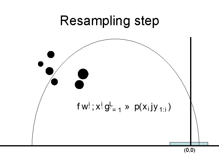
Results in samples one step forward (0, 0)

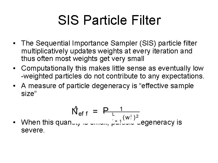
SIS Particle Filter • The Sequential Importance Sampler (SIS) particle filter multiplicatively updates weights at every iteration and thus often most weights get very small • Computationally this makes little sense as eventually low -weighted particles do not contribute to any expectations. • A measure of particle degeneracy is “effective sample size” • When this quantity is small, particle degeneracy is severe.

Solutions • Sequential Importance Re-sampling (SIR) particle filter avoids many of the problems associated with SIS pf’ing by re-sampling the posterior particle set to increase the effective sample size. • Choosing the best possible importance density is also important because it minimizes the variance of the weights which maximizes

Other tricks to improve pf’ing • Integrate out everything you can • Replicate each particle some number of times • In discrete systems, enumerate instead of sample • Use fancy re-sampling schemes like stratified sampling, etc.

Initial particles (0, 0)

Particle evolution step (0, 0)

Weighting step (0, 0)

Resampling step (0, 0)

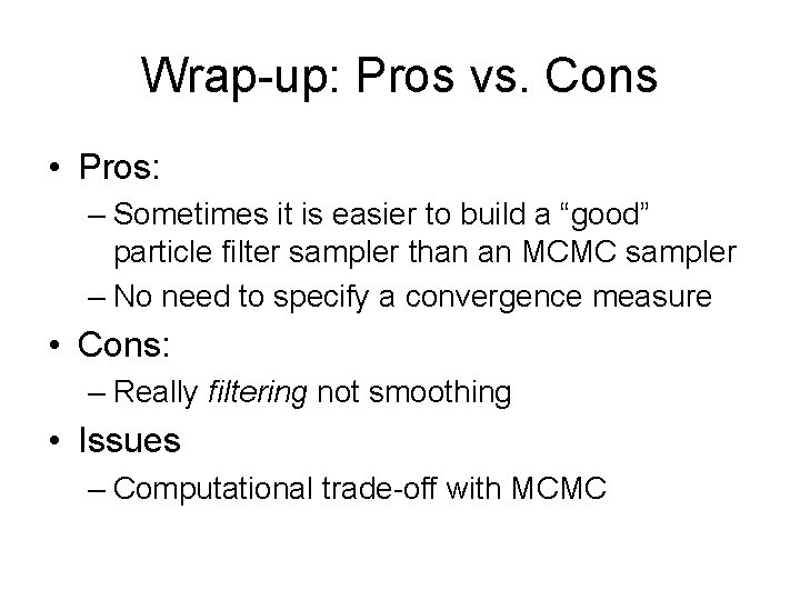
Wrap-up: Pros vs. Cons • Pros: – Sometimes it is easier to build a “good” particle filter sampler than an MCMC sampler – No need to specify a convergence measure • Cons: – Really filtering not smoothing • Issues – Computational trade-off with MCMC

Thank You

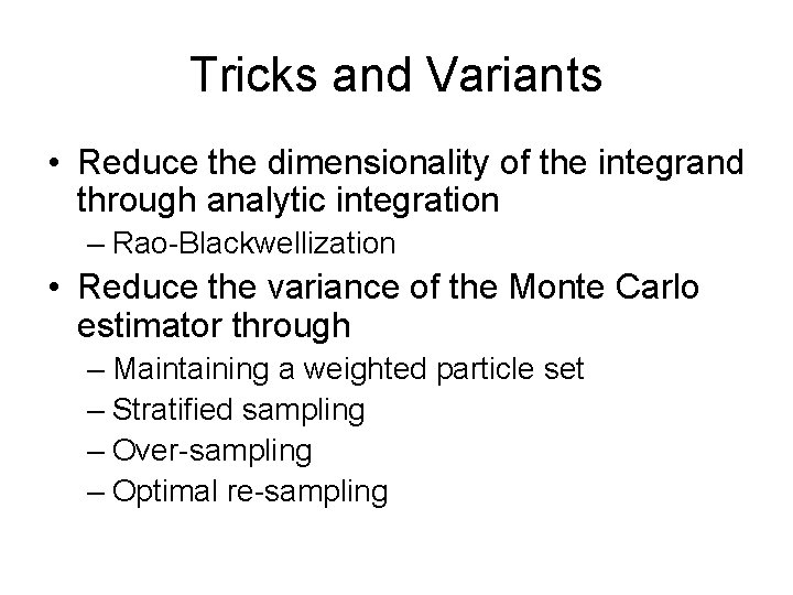
Tricks and Variants • Reduce the dimensionality of the integrand through analytic integration – Rao-Blackwellization • Reduce the variance of the Monte Carlo estimator through – Maintaining a weighted particle set – Stratified sampling – Over-sampling – Optimal re-sampling

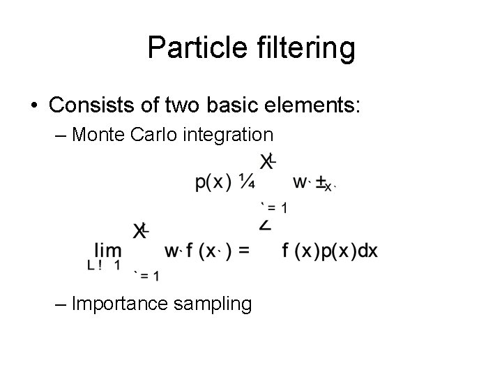
Particle filtering • Consists of two basic elements: – Monte Carlo integration – Importance sampling

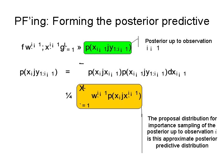
PF’ing: Forming the posterior predictive Posterior up to observation The proposal distribution for importance sampling of the posterior up to observation i is this approximate posterior predictive distribution

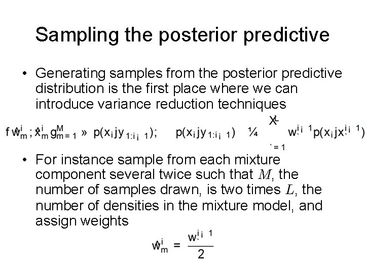
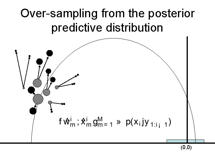
Sampling the posterior predictive • Generating samples from the posterior predictive distribution is the first place where we can introduce variance reduction techniques • For instance sample from each mixture component several twice such that M, the number of samples drawn, is two times L, the number of densities in the mixture model, and assign weights

Not the best • Most efficient Monte Carlo estimator of a function ¡(x) – From survey sampling theory: Neyman allocation – Number drawn from each mixture density is proportional to the weight of the mixture density times the std. dev. of the function ¡ over the mixture density • Take home: smarter sampling possible [Cochran 1963]

Over-sampling from the posterior predictive distribution (0, 0)

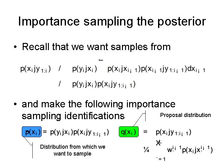
Importance sampling the posterior • Recall that we want samples from • and make the following importance Proposal distribution sampling identifications Distribution from which we want to sample

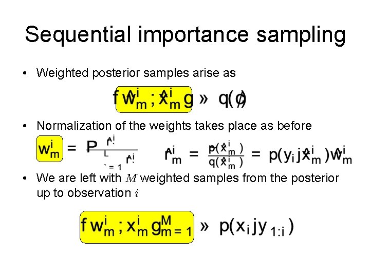
Sequential importance sampling • Weighted posterior samples arise as • Normalization of the weights takes place as before • We are left with M weighted samples from the posterior up to observation i

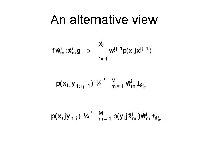
An alternative view

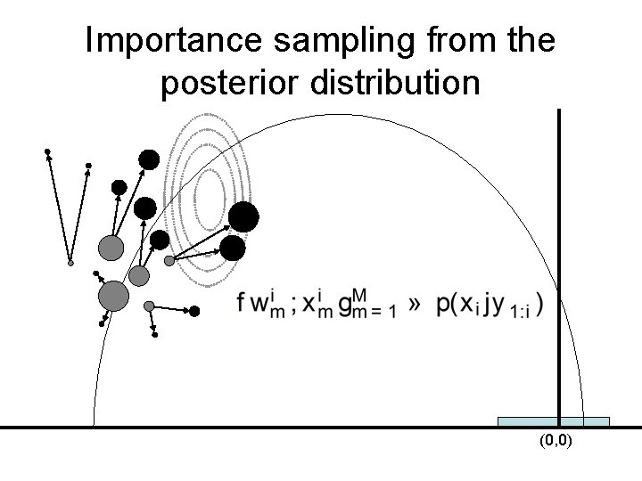
Importance sampling from the posterior distribution (0, 0)

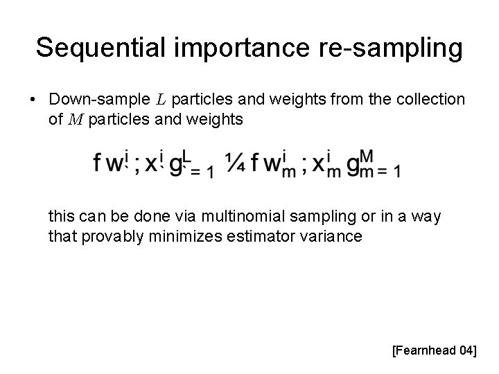
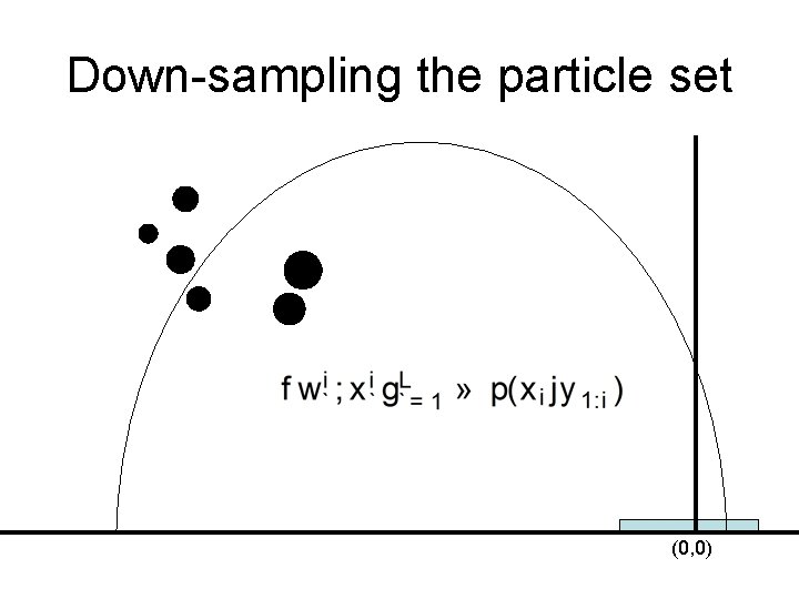
Sequential importance re-sampling • Down-sample L particles and weights from the collection of M particles and weights this can be done via multinomial sampling or in a way that provably minimizes estimator variance [Fearnhead 04]

Down-sampling the particle set (0, 0)

Recap • Starting with (weighted) samples from the posterior up to observation i-1 • Monte Carlo integration was used to form a mixture model representation of the posterior predictive distribution • The posterior predictive distribution was used as a proposal distribution for importance sampling of the posterior up to observation i • M > L samples were drawn and re-weighted according to the likelihood (the importance weight), then the collection of particles was down -sampled to L weighted samples

LSSM Not alone • Various other models are amenable to sequential inference, Dirichlet process mixture modelling is another example, dynamic Bayes’ nets are another

Rao-Blackwellization • In models where parameters can be analytically marginalized out, or the particle state space can otherwise be collapsed, the efficiency of the particle filter can be improved by doing so

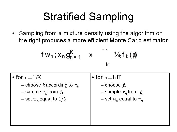
Stratified Sampling • Sampling from a mixture density using the algorithm on the right produces a more efficient Monte Carlo estimator • for n=1: K – choose k according to ¼k – sample xn from fk – set wn equal to 1/N • for n=1: K – choose fn – sample xn from fn – set wn equal to ¼n

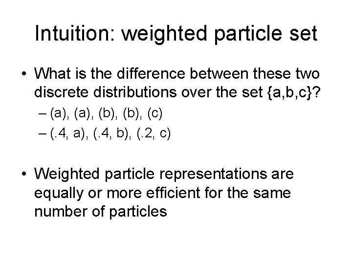
Intuition: weighted particle set • What is the difference between these two discrete distributions over the set {a, b, c}? – (a), (b), (c) – (. 4, a), (. 4, b), (. 2, c) • Weighted particle representations are equally or more efficient for the same number of particles

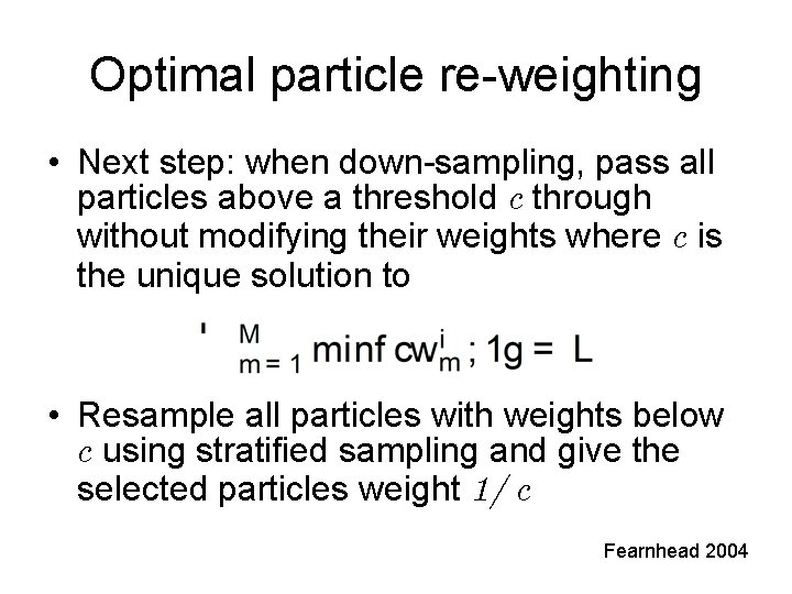
Optimal particle re-weighting • Next step: when down-sampling, pass all particles above a threshold c through without modifying their weights where c is the unique solution to • Resample all particles with weights below c using stratified sampling and give the selected particles weight 1/ c Fearnhead 2004

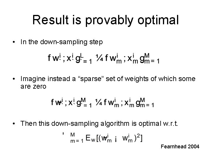
Result is provably optimal • In the down-sampling step • Imagine instead a “sparse” set of weights of which some are zero • Then this down-sampling algorithm is optimal w. r. t. Fearnhead 2004

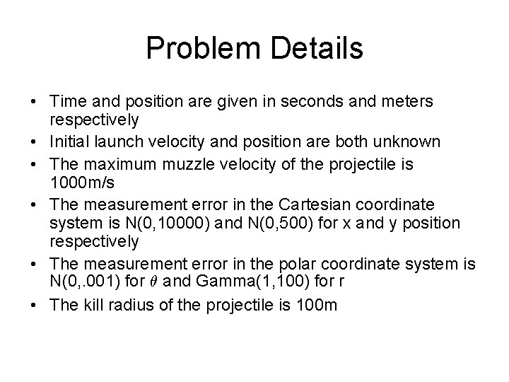
Problem Details • Time and position are given in seconds and meters respectively • Initial launch velocity and position are both unknown • The maximum muzzle velocity of the projectile is 1000 m/s • The measurement error in the Cartesian coordinate system is N(0, 10000) and N(0, 500) for x and y position respectively • The measurement error in the polar coordinate system is N(0, . 001) for µ and Gamma(1, 100) for r • The kill radius of the projectile is 100 m

Data and Support Code http: //www. gatsby. ucl. ac. uk/~fwood/pf_tutorial/

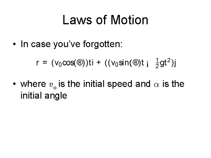
Laws of Motion • In case you’ve forgotten: • where v 0 is the initial speed and ® is the initial angle

Good luck!

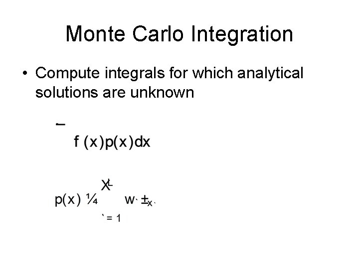
Monte Carlo Integration • Compute integrals for which analytical solutions are unknown

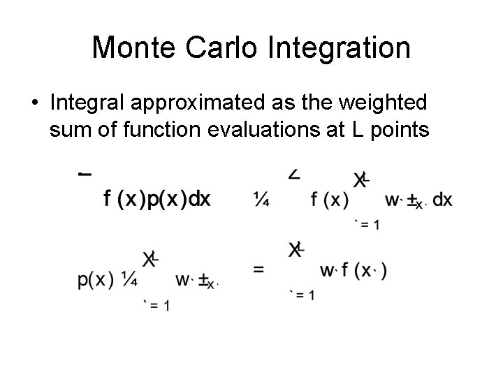
Monte Carlo Integration • Integral approximated as the weighted sum of function evaluations at L points

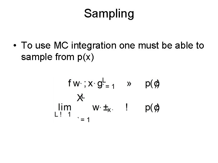
Sampling • To use MC integration one must be able to sample from p(x)

Theory (Convergence) • Quality of the approximation independent of the dimensionality of the integrand • Convergence of integral result to the “truth” is O(1/n 1/2) from L. L. N. ’s. • Error is independent of dimensionality of x

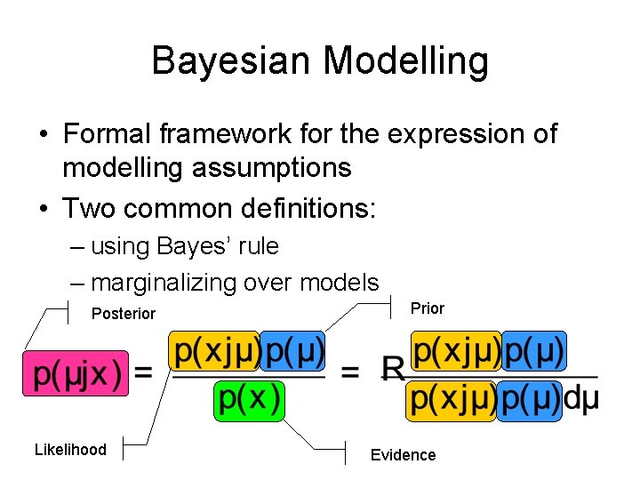
Bayesian Modelling • Formal framework for the expression of modelling assumptions • Two common definitions: – using Bayes’ rule – marginalizing over models Posterior Likelihood Prior Evidence

Posterior Estimation • Often the distribution over latent random variables (parameters) is of interest • Sometimes this is easy (conjugacy) • Usually it is hard because computing the evidence is intractable

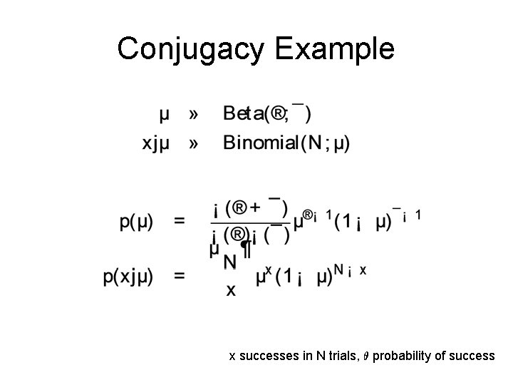
Conjugacy Example x successes in N trials, µ probability of success

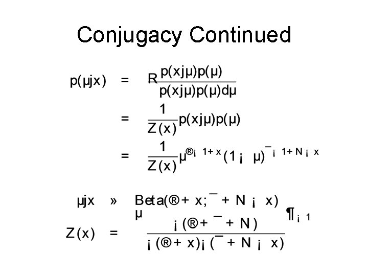
Conjugacy Continued

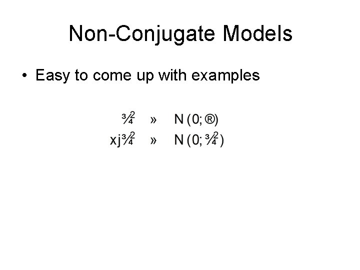
Non-Conjugate Models • Easy to come up with examples

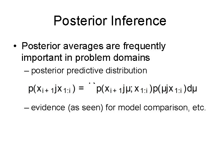
Posterior Inference • Posterior averages are frequently important in problem domains – posterior predictive distribution – evidence (as seen) for model comparison, etc.

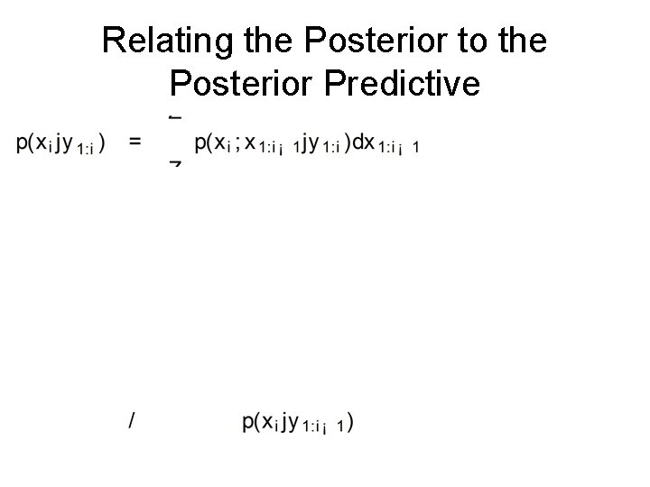
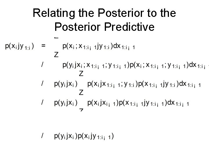
Relating the Posterior to the Posterior Predictive

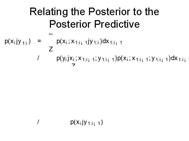
Relating the Posterior to the Posterior Predictive

Relating the Posterior to the Posterior Predictive

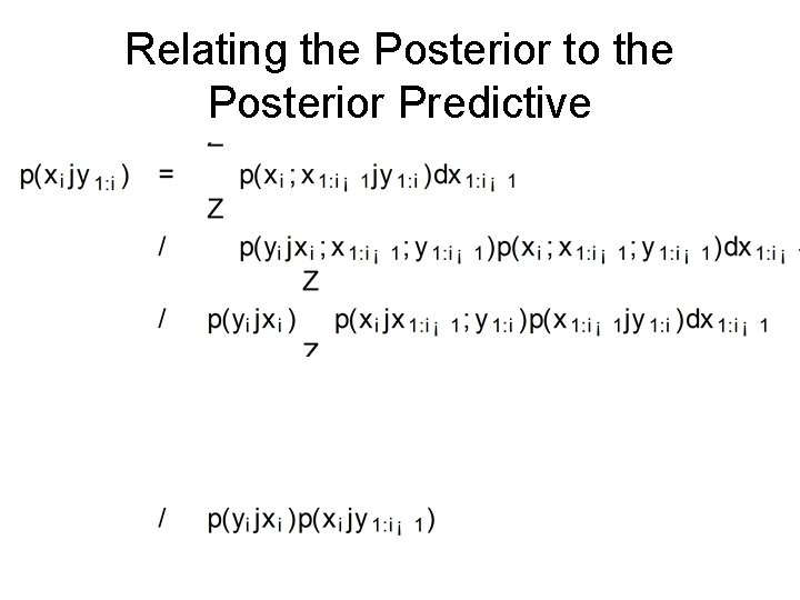
Relating the Posterior to the Posterior Predictive

Importance sampling Proposal distribution: easy to sample from Original distribution: hard to sample from, easy to evaluate Importance weights

Importance sampling un-normalized distributions Un-normalized distribution to sample from, still hard to sample from and easy to evaluate Un-normalized proposal distribution: still easy to sample from New term: ratio of normalizing constants

Normalizing the importance weights Un-normalized importance weights Normalized importance weights Takes a little algebra

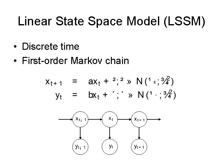
Linear State Space Model (LSSM) • Discrete time • First-order Markov chain

Inferring the distributions of interest • Many methods exist to infer these distributions – – Markov Chain Monte Carlo (MCMC) Variational inference Belief propagation etc. • In this setting sequential inference is possible because of characteristics of the model structure and preferable due to the problem requirements

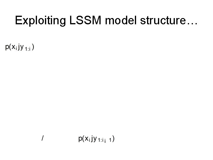
Exploiting LSSM model structure…

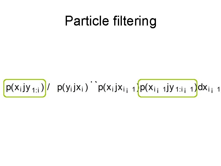
Particle filtering

Exploiting Markov structure… Use Bayes’ rule and the conditional independence structure dictated by the first order Markov hidden variable model

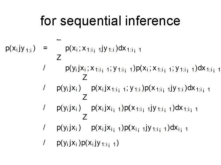
for sequential inference

An alternative view

Sequential importance sampling inference • Start with a discrete representation of the posterior up to observation i-1 • Use Monte Carlo integration to represent the posterior predictive distribution as a finite mixture model • Use importance sampling with the posterior predictive distribution as the proposal distribution to sample the posterior distribution up to observation i

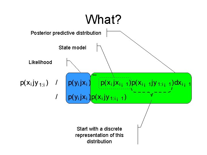
What? Posterior predictive distribution State model Likelihood Start with a discrete representation of this distribution

Monte Carlo integration General setup As applied in this stage of the particle filter Samples from Finite mixture model