Sequencing and Assembly GEN 875 Genomics and Proteomics

Sequencing and Assembly GEN 875, Genomics and Proteomics, Fall 2010

Adapted from Francis Oulette; Adapted from Eric Green, NIH; Adapted from Messing & Llaca, PNAS (1998) History of DNA Sequencing 1870 Miescher: Discovers DNA 1940 Avery: Proposes DNA as ‘Genetic Material’ Efficiency (bp/person/year) 1953 Watson & Crick: Double Helix Structure of DNA 1 1965 Holley: Sequences Yeast t. RNAAla 1970 Wu: Sequences Cohesive End DNA 1977 Sanger: Dideoxy Chain Termination Gilbert: Chemical Degradation 1980 Messing: M 13 Cloning 1986 Hood et al. : Partial Automation 15 150 1, 500 15, 000 25, 000 50, 000 1990 • Cycle Sequencing • Improved Sequencing Enzymes • Improved Fluorescent Detection Schemes 200, 000 50, 000 100, 000, 000 2002 2008 • Next Generation Sequencing • Improved enzymes and chemistry • Improved image processing

Explosive Growth in Sequencing 8/22/2005 Press Release: INSD (Gen. Bank, EMBL, DDBJ) reaches 100 Gigabase milestone

What do we sequence? • • Genomes (de novo, resequencing) Metagenomes or complex samples Transcripts Fragments recovered by ch. IP or tagged in some other way

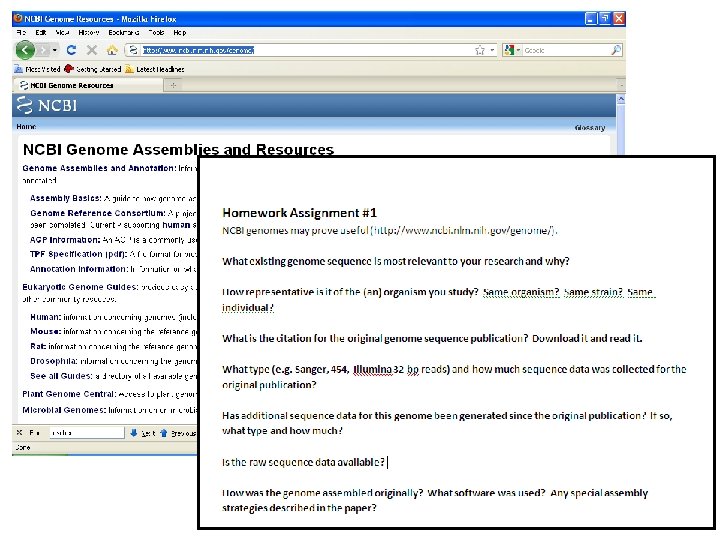
NCBI Genomes http: //www. ncbi. nlm. nih. gov/Genomes/ Comparison of data from 9/4/08, 9/5/07, 9/4/06 and 8/31/05 Eukaryotic Genomes: Complete Assembly In progress 23, 25, 22, 20 230, 162, 109, 72 229, 235, 299, 166 Prokaryotic Genomes: Complete In progress 745, 567, 371, 254 1215, 841, 615, 433

NCBI Genomes 9/6/2010

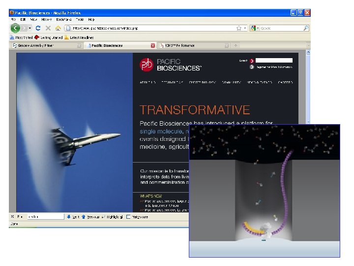
Sequencing Platforms • Sanger sequencing and capillary electrophoresis • Massively parallel pyrosequencing (454) • “proprietary Clonal Single Molecule Array technology and novel reversible terminatorbased sequencing” (Illumina) • Sequencing by ligation (ABI SOLi. D) • Single molecule sequencing (Pac. Bio)

Basics of the “old” technology • Clone the DNA. • Generate a ladder of labeled (colored) molecules that are different by 1 nucleotide. • Separate mixture on some matrix. • Detect fluorochrome by laser. • Interpret peaks as string of DNA. • Strings are 500 to 1, 000 letters long • 1 machine generates 57, 000 nucleotides/run • Assemble all strings into a genome. Adapted from Francis Oulette

Library construction and sequencing High-throughput Steps Sample Isolate DNA Cycle Sequencing Size selection Physical fragmentation Isolate cloned constructs Ligate randomly into vectors Transformation Pick and grow individual colonies Plate on agar

Dual Ended Sequencing Can Provide Information to Link Contigs Sequencing with primers that begin in the vector on either side of the insert yields about 800 bp of DNA sequence from each end of the insert 5 Kb insert Primer A Primer B The middle of the insert is never sequenced for most clones used in the project

Basics of the “new” technology • • Get DNA. Attach it to something. Extend amplify signal with some labeling scheme. Detect fluorochrome by microscopy. Interpret series of spots as short strings of DNA. Strings are 30 -300 letters long Multiple images are interpreted as 0. 4 to 1. 2 GB/run (1, 200, 000 letters/day). • Map or align strings to one or many genome or assemble. Adapted from Francis Oulette

Differences between the various platforms: • • • Nanotechnology used. Resolution of the image analysis. Chemistry and enzymology. Signal to noise detection in the software Software/images/file size/pipeline Cost $$$ Adapted from Francis Oulette

Adapted from Richard Wilson, School of Medicine, Washington University, “Sequencing the Cancer Genome” http: //tinyurl. com/5 f 3 alk Next Generation DNA Sequencing Technologies 3 Gb ==

Roche 454 Pyrosequencing Genome sequencing in microfabricated high-density picolitre reactors Margulies, M. Eghold, M. et al. Nature. 2005 Sep 15; 437(7057): 326 -7

GS FLX Titanium Series: Throughput 400 -600 million high-quality, filter-passed bases per run* 1 billion bases per day Run Time 10 hours Read Length Average length = 400 bases Accuracy Q 20 read length of 400 bases (99% at 400 bases and higher for prior bases) Reads per run >1 million high-quality reads

Adapted from Richard Wilson, School of Medicine, Washington University, “Sequencing the Cancer Genome” http: //tinyurl. com/5 f 3 alk Solexa-based Whole Genome Sequencing

Adapted from Richard Wilson, School of Medicine, Washington University, “Sequencing the Cancer Genome” http: //tinyurl. com/5 f 3 alk Solexa-based Whole Genome Sequencing Solexa flow cell ~50 M clusters are sequenced per flow cell.

Debbie Nickerson, Department of Genome Sciences, University of Washington, http: //tinyurl. com/6 zbzh 4

Genome-scale Sequence Analysis • De novo assembly • Templated assembly • Read mapping or alignment to a reference genome

“The choice of alignment or assembly algorithm is strongly influenced by both the experiment in question and the details of the sequencing technology used. The performance characteristics of the sequencing machines are changing rapidly, and any delineation of performance characteristics such as machine capacity, run time or read length and its relationship to error profile will quickly be outdated. ”

Assemblers • Greedy Assemblers – compare all reads to each other then join them in order of overlap size Figure 8. Greedy assembly of four reads.

Assemblers • Overlap Graph Assemblers – make a graph where each node represents a read and edges between them represent overlaps. Figure 9. Overlap graph for a bacterial genome. The thick edges in the picture on the left (a Hamiltonian cycle) correspond to the correct layout of the reads along the genome (figure on the right). The remaining edges represent false overlaps induced by repeats (exemplified by the red lines in the figure on the right)

Assembly with dual-ended sequencing Sequence assembly Contigs joined by overlaps Contigs linked by a spanning clone Scaffold – two or more linked contigs

Repeat handling • Screen out known repeats and set them aside for later • Infer repetitiveness based on coverage • First assemble unambiguous overlaps, then resolve repeats using mate pairs

Assemblers and short reads • Full overlap assemblers compare all reads against all other reads. Scale quadratically with the number of reads. • Computationally intractable for large NSG datasets • Led to development of k-mer based methods: a de Bruijn graph with a node for every k-mer observed in the sequence set and an edge between nodes if these two k-mers are observed adjacently in a read

Figure 2. Differences between an overlap graph and a de Bruijn graph for assembly. Based on the set of 10 8 -bp reads (A), we can build an overlap graph (B) in which each read is a node, and overlaps >5 bp are indicated by directed edges. Transitive overlaps, which are implied by other longer overlaps, are shown as dotted edges. In a de Bruin graph (C ), a node is created for every k-mer in all the reads; here the k-mer size is 3. Edges are drawn between every pair of successive k-mers in a read, where the k-mers overlap by k 1 bases. In both approaches, repeat sequences create a fork in the graph. Note here we have only considered the forward orientation of each sequence to simplify the figure.

Figure 1. The k-mer uniqueness ratio for five well-known organisms and one single-celled human parasite. The ratio is defined here as the percentage of the genome that is covered by unique sequences of length k or longer. The horizontal axis shows the length in base pairs of the sequences. For example, ; 92. 5% of the grapevine genome is contained in unique sequences of 100 bp or longer.

De Bruijn k-mer assemblers • Newbler (Roche 454) • SHARCGS • VCAKE • VELVET • EULER-SR • EDENA • ABy. SS • ALLPATHS • SOAPdenovo • Contrail

• Most assemblers have an error detection and resolution phase • Errors produce characteristic graphic structures

Problems with de Bruijn graph methods • Require large amount of memory to store graph – for example Velvet would require a terabyte of memory to assemble the human genome • Not as easy to parallelize as overlap assemblers From Shatz et al. 2010: “To date, only two de Bruijn graph assemblers have been shown to have the ability to assemble a mammalian-sized genome. ABy. SS (Simpson et al. 2009) assembled a human genome in 87 h on a cluster of 21 eight-core machines each with 16 GB of RAM (168 cores, 336 GB of RAM total). SOAPdenovo assembled a human genome in 40 h using a single computer with 32 cores and 512 GB of RAM (Li et al. 2010). Although these types of computing resources are not widely available, they are within reach for large-scale scientific centers. ”

How many clones/reads do we need? …according to the work of Lander and Waterman (Genomic mapping by fingerprinting random clones: a mathematical analysis. Genomics. 1988 the number of “islands” or contigs formed from randomly collected sequences depends on: Apr; 2(3): 231 -9. ), G L N T = = Genome Length Sequence Read Length Number of Sequences Collected Number of Basepairs of Overlap Needed (# Islands = Ne LN G (1 - T L ))

5 Mbp Genome, 500 bp reads, 25 bp overlap • • • • # reads 2500 5000 10000 20000 30000 40000 50000 60000 70000 80000 90000 100000 coverage 0. 25 0. 5 1 2 3 4 5 6 7 8 9 10 % sequenced 22. 12 39. 35 63. 21 86. 47 95. 02 98. 17 99. 33 99. 75 99. 91 99. 97 99. 99 100. 00 # contigs 1971 3109 3867 2991 1735 895 433 201 91 40 17 7

Graph of previous data

Genome size as predicted from the assembly # non-singleton contigs 2500 Shotgun Sequencing Model 2000 Predicted 5. 5 Mb size Observed # non-singletons 1500 Predicted 3. 7 Mb size 1000 500 0 0 10, 000 20, 000 30, 000 # Sequences 40, 000 50, 000 60, 000 70, 000

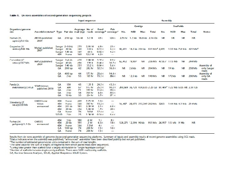
Figure 3. Expected average contig length for a range of different read lengths and coverage values. Also shown are the average contig lengths and N 50 lengths for the dog genome, assembled with 710 -bp reads, and the panda genome, assembled with reads averaging 52 bp in length.

Combining sequence data types • In practice, appears to be the best strategy for both microbial and eukaryotic genomes • Creates assembly challenges of its own

One strategy for microbial genomes • ~¼ run of 454 regular, ¼ run of paired end (2. 5 kb library) plus one lane of Solexa • Assemble Solexa data with Velvet • Assemble 454 data with Newbler • Shred the Velvet assembly into Newbler size reads and add it to the 454 assembly • Use Solexa deep coverage to “polish”

Gap Closure Strategies • Primer walk to sequence the rest of linking clones that span a scaffold gap • Primer walk off clones at the ends of contigs for which there is no linking information • PCR based on your best guess at contig order (comparison to other closely related genomes, predicted genes at the end of genomes, anything else you can come up with) • Combinatorial PCR with primers designed at the end of each contig

Phred Scores Phred Score P( incorrect base ) Base call accuracy 10 1 in 10 90% 20 1 in 100 99% 30 1 in 1000 99. 9% 40 1 in 10000 99. 99% 50 1 in 100000 99. 999%