SEPARATING CATCHUP AND TECHNICAL CHANGE IN STOCHASTIC FRONTIER

SEPARATING CATCH-UP AND TECHNICAL CHANGE IN STOCHASTIC FRONTIER MODELS. A MONTE CARLO APPROACH Julio del Corral Antonio Álvarez University of Oviedo XXXIII SAE 11 -13 December, 2008 Zaragoza

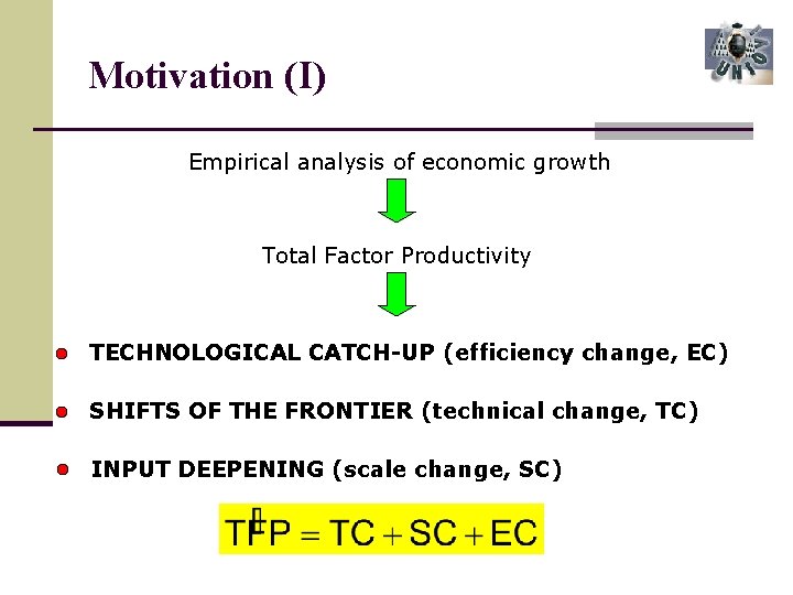
Motivation (I) Empirical analysis of economic growth Total Factor Productivity TECHNOLOGICAL CATCH-UP (efficiency change, EC) SHIFTS OF THE FRONTIER (technical change, TC) INPUT DEEPENING (scale change, SC)

Motivation (II) Two approaches of TFP changes decomposition: Non-parametric models: Compute Malmquist productivity indexes using DEA e. g. Färe et al. (1994), Kumar and Rusell (2002) Parametric models: Stochastic frontiers with time varying efficiency e. g. Koop et al. (1999), Kumbhakar and Wang (2005)

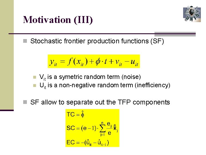
Motivation (III) n Stochastic frontier production functions (SF) n n Vit is a symetric random term (noise) Uit is a non-negative random term (inefficiency) n SF allow to separate out the TFP components

Motivation (IV) n Important n Both TC and EC (catch-up) are non observable n Both are modelled as time functions n Difficulty “It may be difficult to disentangle the separate effects of technical change and technical efficiency change when both effects are proxied by the passage of time” n Kumbhakar and Lovell (2000)

Objetive To study the ability of several stochastic frontier models to correctly identify technical change and efficiency change By using Monte Carlo techniques we compare several stochastic frontier models

Monte Carlo design (I) Our experiments are based on a realistic configuration of the right-hand side of the estimated equation, rather than simply simulating some small number of artificial regressors We take input variables (capital and labor) from the Penn World Table 6. 2 91 countries, 31 years (1970 -2000)

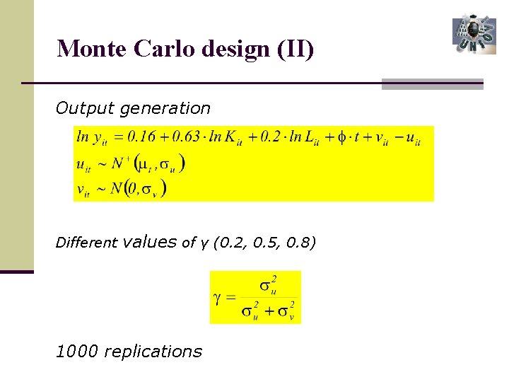
Monte Carlo design (II) Output generation Different values of γ (0. 2, 0. 5, 0. 8) 1000 replications

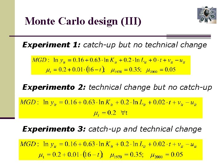
Monte Carlo design (III) Experiment 1: catch-up but no technical change Experimento 2: technical change but no catch-up Experimento 3: catch-up and technical change

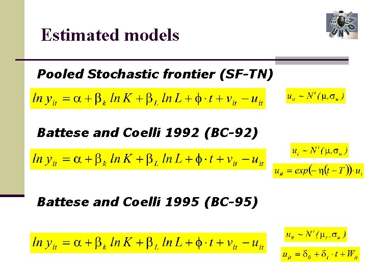
Estimated models Pooled Stochastic frontier (SF-TN) Battese and Coelli 1992 (BC-92) Battese and Coelli 1995 (BC-95)

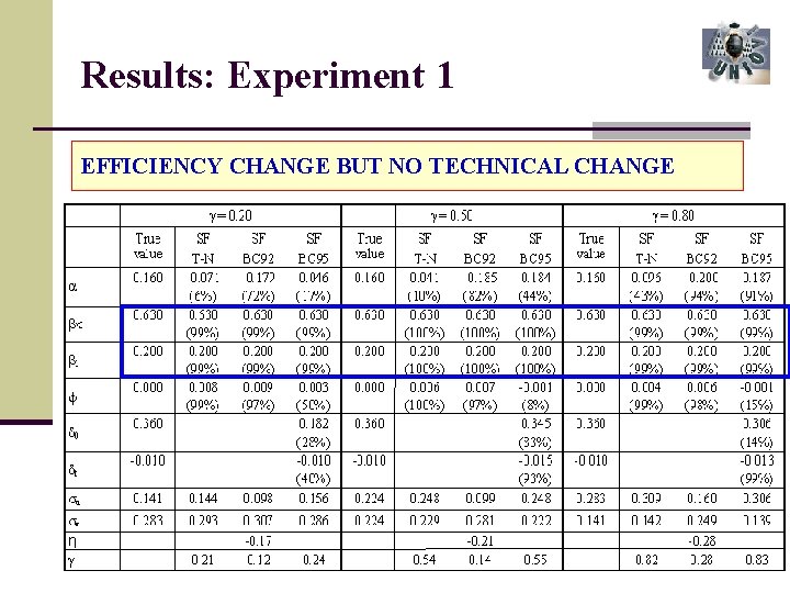
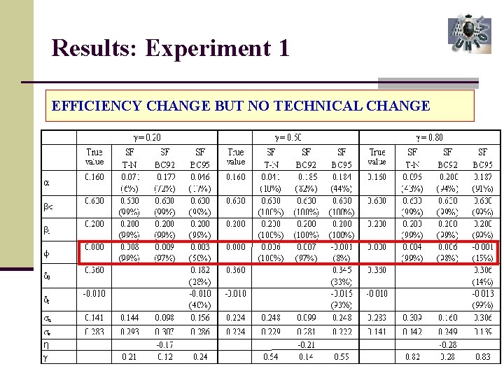
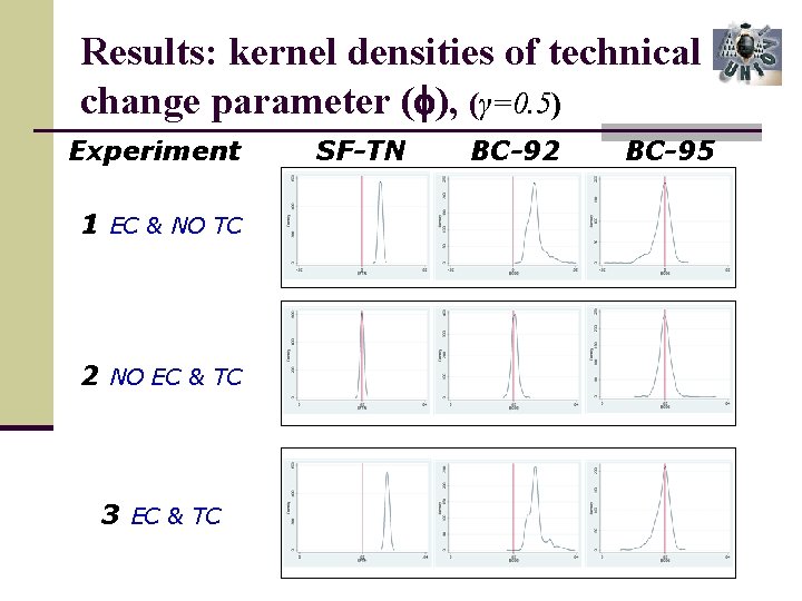
Results: Experiment 1 EFFICIENCY CHANGE BUT NO TECHNICAL CHANGE

Results: Experiment 1 EFFICIENCY CHANGE BUT NO TECHNICAL CHANGE

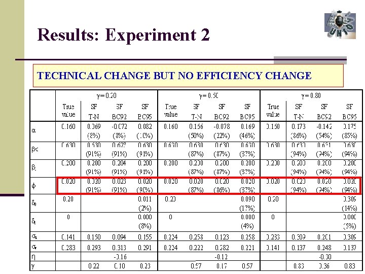
Results: Experiment 2 TECHNICAL CHANGE BUT NO EFFICIENCY CHANGE

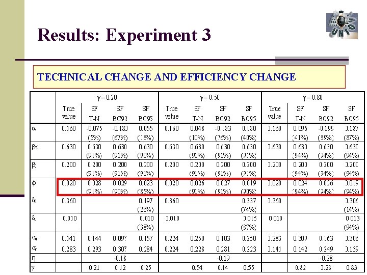
Results: Experiment 3 TECHNICAL CHANGE AND EFFICIENCY CHANGE

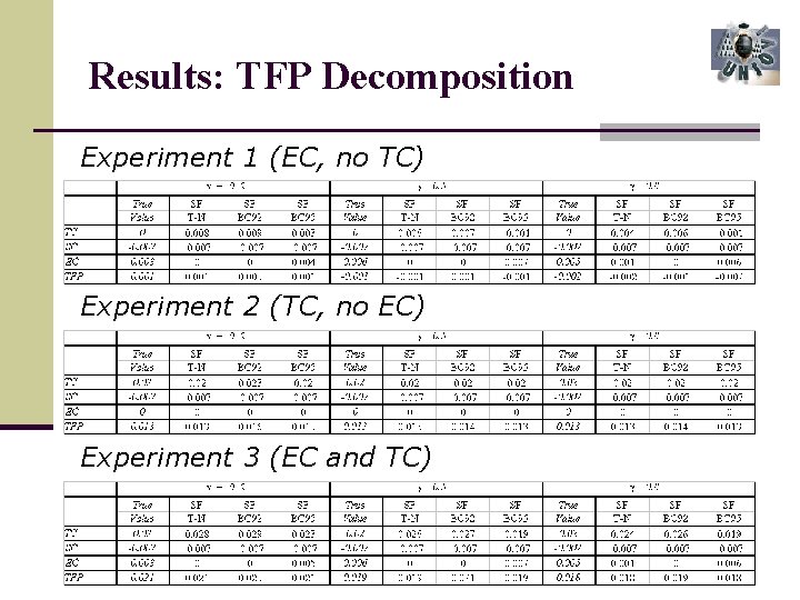
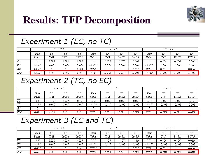
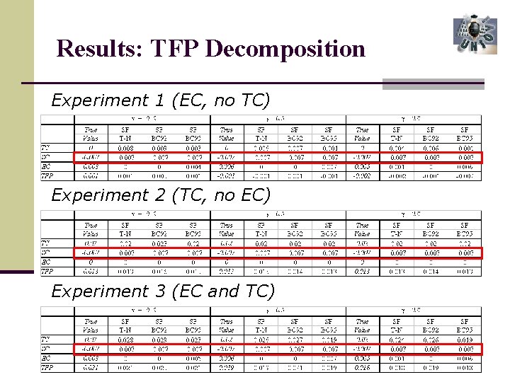
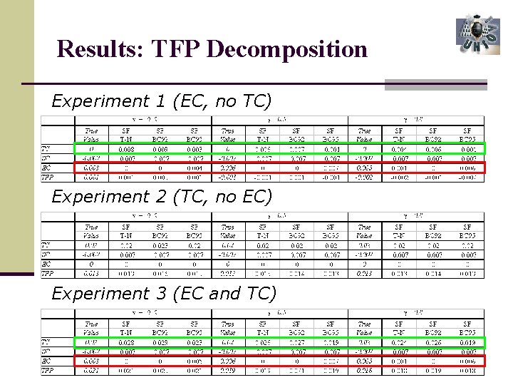
TFP change decomposition Experiment 1: EC & NO TC (γ=0, 8) True SF SF SF Value T-N BC 92 BC 95 TC 0 0. 004 0. 006 -0. 001 SC -0. 007 EC 0. 005 0. 001 0. 000 0. 006 TFP -0. 002 -0. 001 -0. 002

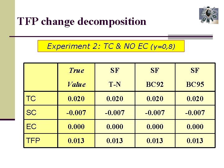
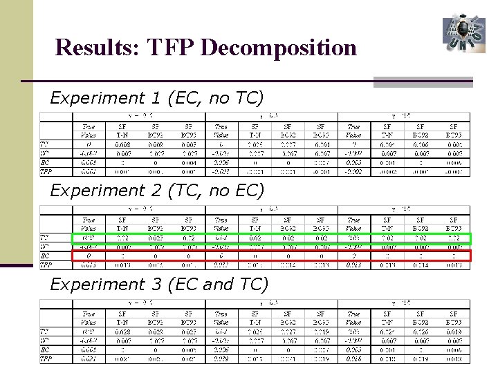
TFP change decomposition Experiment 2: TC & NO EC (γ=0, 8) True SF SF SF Value T-N BC 92 BC 95 TC 0. 020 SC -0. 007 EC 0. 000 TFP 0. 013

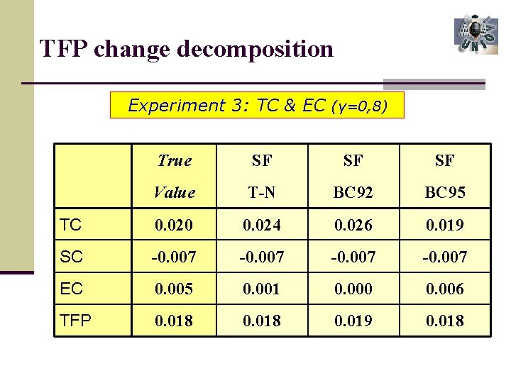
TFP change decomposition Experiment 3: TC & EC (γ=0, 8) True SF SF SF Value T-N BC 92 BC 95 TC 0. 020 0. 024 0. 026 0. 019 SC -0. 007 EC 0. 005 0. 001 0. 000 0. 006 TFP 0. 018 0. 019 0. 018

Results: kernel densities of technical change parameter ( ), (γ=0. 5) Experiment 1 EC & NO TC 2 NO EC & TC 3 EC & TC SF-TN BC-92 BC-95

Thanks a lot for your attention!! Comments welcome at corraljulio@uniovi. es

Results: TFP Decomposition Experiment 1 (EC, no TC) Experiment 2 (TC, no EC) Experiment 3 (EC and TC)

Results: TFP Decomposition Experiment 1 (EC, no TC) Experiment 2 (TC, no EC) Experiment 3 (EC and TC)

Results: TFP Decomposition Experiment 1 (EC, no TC) Experiment 2 (TC, no EC) Experiment 3 (EC and TC)

Results: TFP Decomposition Experiment 1 (EC, no TC) Experiment 2 (TC, no EC) Experiment 3 (EC and TC)

Results: TFP Decomposition Experiment 1 (EC, no TC) Experiment 2 (TC, no EC) Experiment 3 (EC and TC)