Sensitivity Analysis Consider the Cross Chek hockey stick

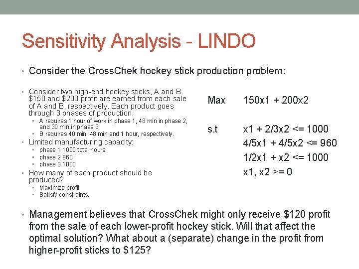
Sensitivity Analysis • Consider the Cross. Chek hockey stick production problem: • Consider two high-end hockey sticks, A and B. $150 and $200 profit are earned from each sale of A and B, respectively. Each product goes through 3 phases of production. • A requires 1 hour of work in phase 1, 48 min in phase 2, and 30 min in phase 3. • B requires 40 min, 48 min and 1 hour, respectively. • Limited manufacturing capacity: • phase 1 1000 total hours • phase 2 960 • phase 3 1000 • How many of each product should be produced? • Maximize profit • Satisfy constraints. Max s. t 150 x 1 + 200 x 2 x 1 + 2/3 x 2 <= 1000 4/5 x 1 + 4/5 x 2 <= 960 1/2 x 1 + x 2 <= 1000 x 1, x 2 >= 0 • Management believes that Cross. Chek might only receive $120 profit from the sale of each lower-profit hockey stick. Will that affect the optimal solution? What about a (separate) change in the profit from higher-profit sticks to $125?

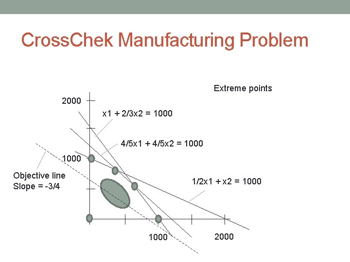
Cross. Chek Manufacturing Problem 2000 x 1 + 2/3 x 2 = 1000 4/5 x 1 + 4/5 x 2 = 1000 Objective line Slope = -3/4 1/2 x 1 + x 2 = 1000 2000

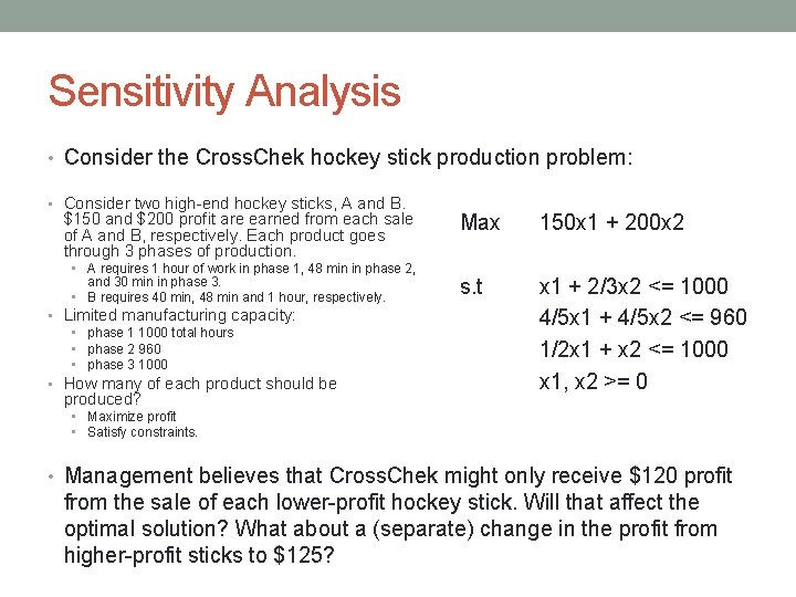
Cross. Chek Manufacturing Problem Extreme points 2000 x 1 + 2/3 x 2 = 1000 4/5 x 1 + 4/5 x 2 = 1000 Objective line Slope = -3/4 1/2 x 1 + x 2 = 1000 2000

Cross. Chek Manufacturing Problem 2000 x 1 + 2/3 x 2 = 1000 4/5 x 1 + 4/5 x 2 = 1000 Objective line Slope = -3/4 1/2 x 1 + x 2 = 1000 2000

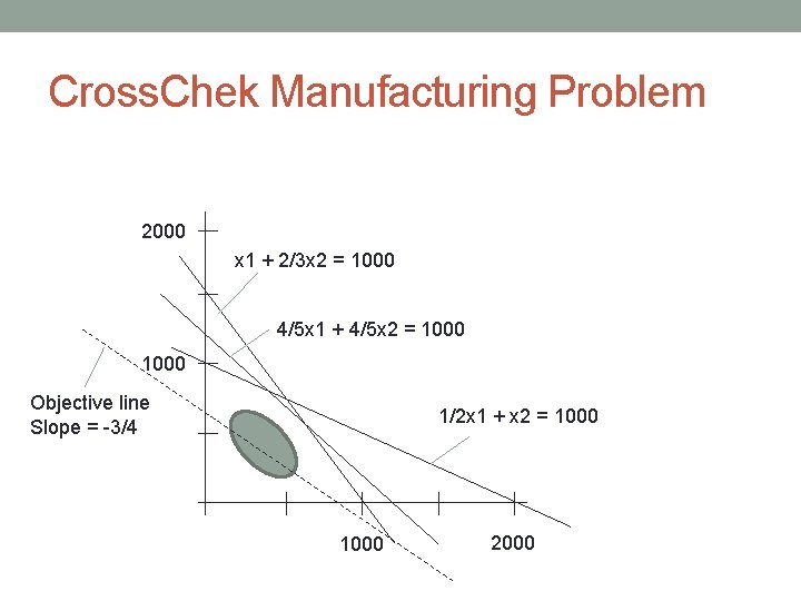
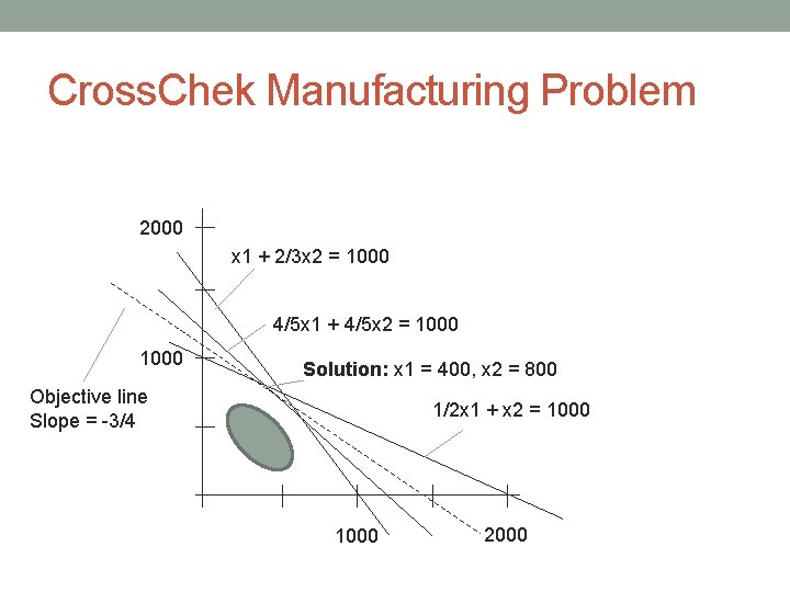
Cross. Chek Manufacturing Problem 2000 x 1 + 2/3 x 2 = 1000 4/5 x 1 + 4/5 x 2 = 1000 Solution: x 1 = 400, x 2 = 800 Objective line Slope = -3/4 1/2 x 1 + x 2 = 1000 2000

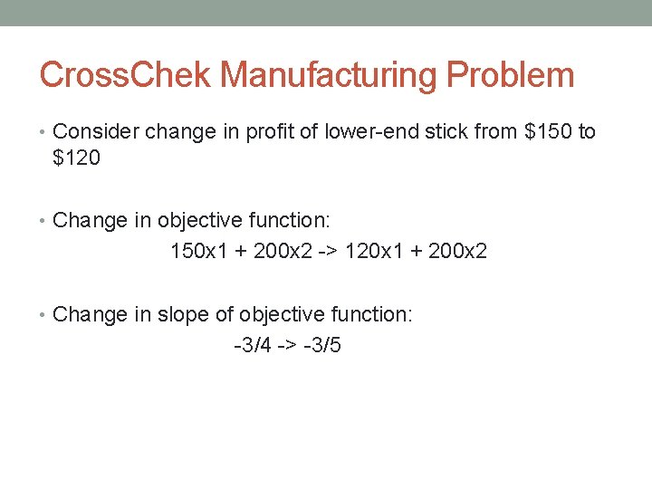
Cross. Chek Manufacturing Problem • Consider change in profit of lower-end stick from $150 to $120 • Change in objective function: 150 x 1 + 200 x 2 -> 120 x 1 + 200 x 2 • Change in slope of objective function: -3/4 -> -3/5

Cross. Chek Manufacturing Problem 2000 x 1 + 2/3 x 2 = 1000 4/5 x 1 + 4/5 x 2 = 1000 Objective line Slope = -3/4 1/2 x 1 + x 2 = 1000 2000

Cross. Chek Manufacturing Problem 2000 x 1 + 2/3 x 2 = 1000 4/5 x 1 + 4/5 x 2 = 1000 Objective line Slope = -3/5 1/2 x 1 + x 2 = 1000 2000

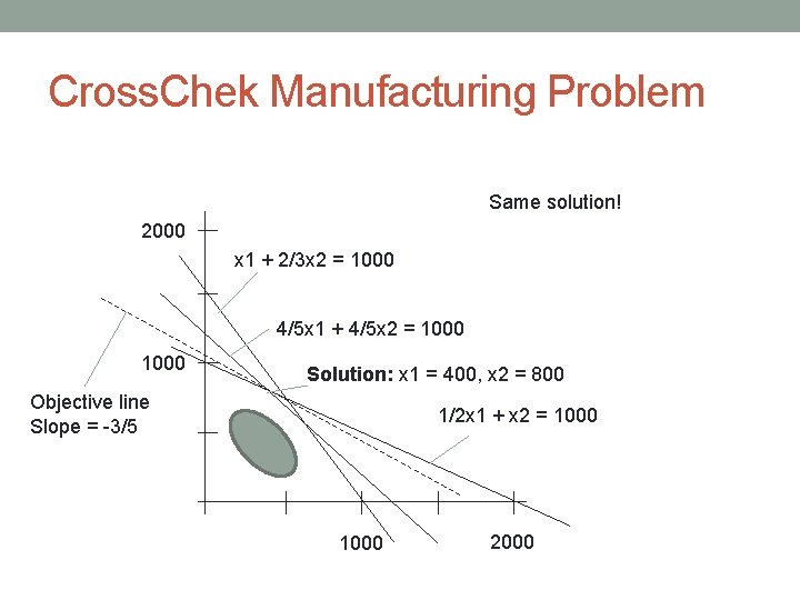
Cross. Chek Manufacturing Problem Same solution! 2000 x 1 + 2/3 x 2 = 1000 4/5 x 1 + 4/5 x 2 = 1000 Solution: x 1 = 400, x 2 = 800 Objective line Slope = -3/5 1/2 x 1 + x 2 = 1000 2000

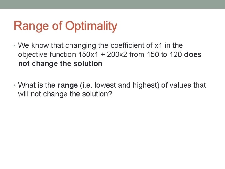
Range of Optimality • We know that changing the coefficient of x 1 in the objective function 150 x 1 + 200 x 2 from 150 to 120 does not change the solution • What is the range (i. e. lowest and highest) of values that will not change the solution?

Range of Optimality 2000 x 1 + 2/3 x 2 = 1000 4/5 x 1 + 4/5 x 2 = 1000 Objective line Slope = -3/4 1/2 x 1 + x 2 = 1000 2000

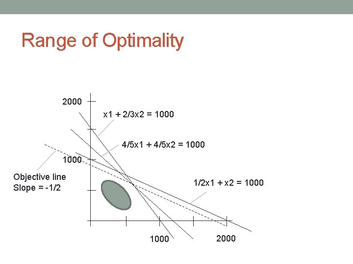
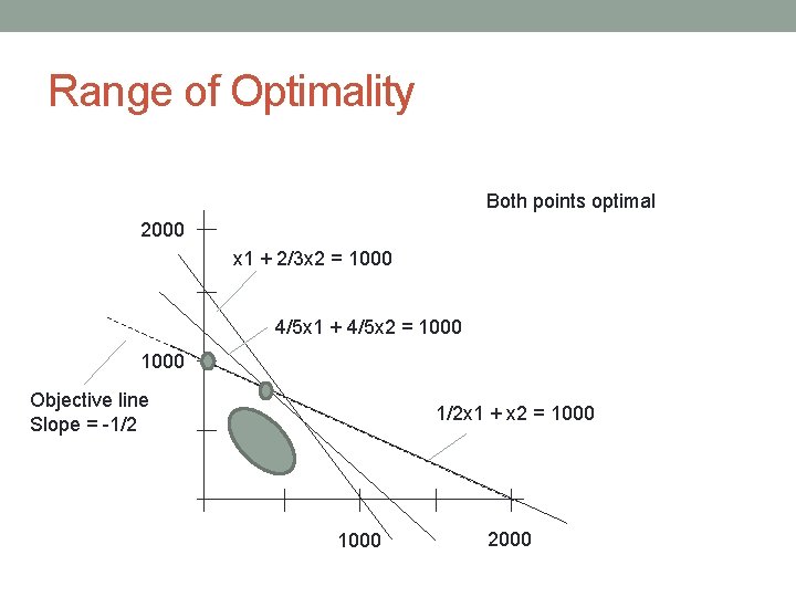
Range of Optimality 2000 x 1 + 2/3 x 2 = 1000 4/5 x 1 + 4/5 x 2 = 1000 Objective line Slope = -1/2 1/2 x 1 + x 2 = 1000 2000

Range of Optimality 2000 x 1 + 2/3 x 2 = 1000 4/5 x 1 + 4/5 x 2 = 1000 Objective line Slope = -1/2 1/2 x 1 + x 2 = 1000 2000

Range of Optimality Both points optimal 2000 x 1 + 2/3 x 2 = 1000 4/5 x 1 + 4/5 x 2 = 1000 Objective line Slope = -1/2 1/2 x 1 + x 2 = 1000 2000

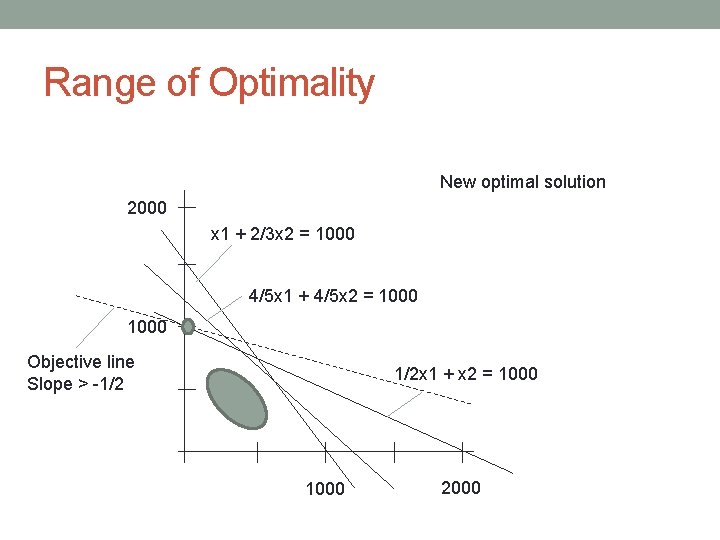
Range of Optimality New optimal solution 2000 x 1 + 2/3 x 2 = 1000 4/5 x 1 + 4/5 x 2 = 1000 Objective line Slope > -1/2 1/2 x 1 + x 2 = 1000 2000

Range of Optimality 2000 x 1 + 2/3 x 2 = 1000 4/5 x 1 + 4/5 x 2 = 1000 Objective line Slope = -3/4 1/2 x 1 + x 2 = 1000 2000

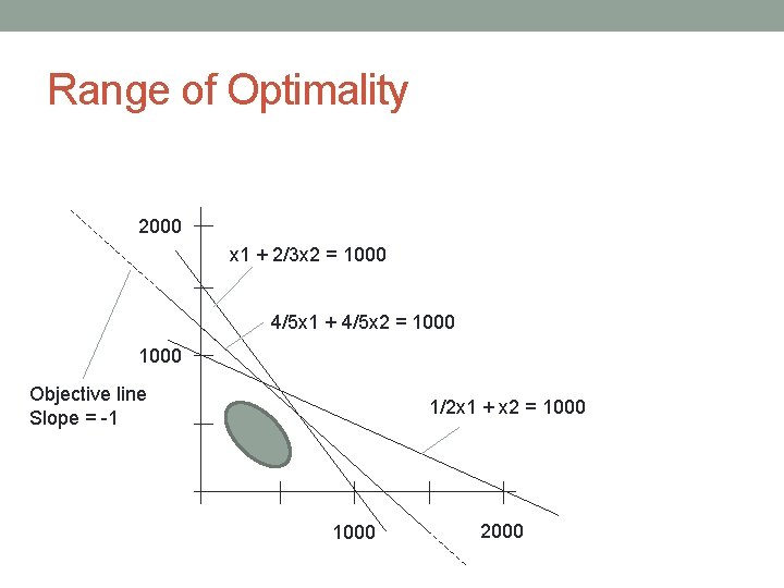
Range of Optimality 2000 x 1 + 2/3 x 2 = 1000 4/5 x 1 + 4/5 x 2 = 1000 Objective line Slope = -1 1/2 x 1 + x 2 = 1000 2000

Range of Optimality 2000 x 1 + 2/3 x 2 = 1000 4/5 x 1 + 4/5 x 2 = 1000 Objective line Slope = -1 1/2 x 1 + x 2 = 1000 2000

Range of Optimality Both points optimal 2000 x 1 + 2/3 x 2 = 1000 4/5 x 1 + 4/5 x 2 = 1000 Objective line Slope = -1 1/2 x 1 + x 2 = 1000 2000

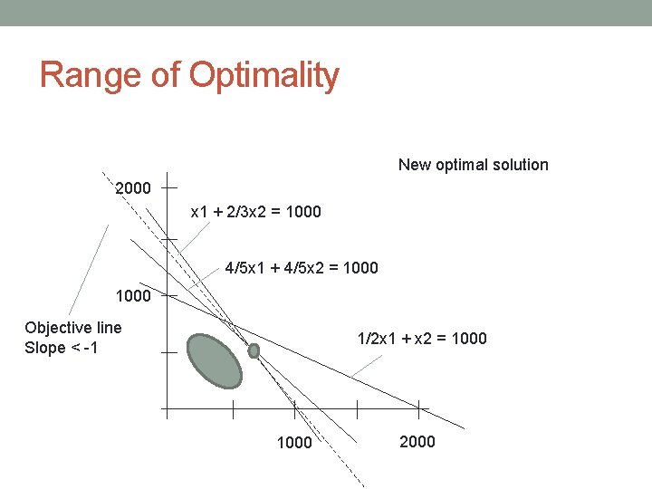
Range of Optimality New optimal solution 2000 x 1 + 2/3 x 2 = 1000 4/5 x 1 + 4/5 x 2 = 1000 Objective line Slope < -1 1/2 x 1 + x 2 = 1000 2000

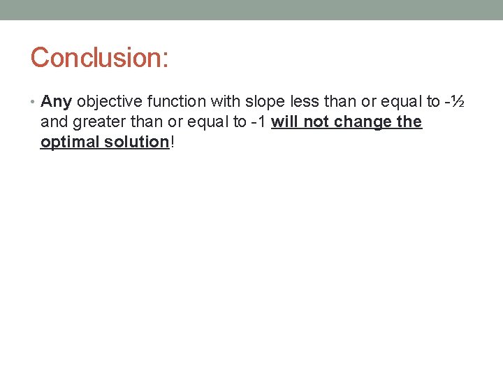
Conclusion: • Any objective function with slope less than or equal to -½ and greater than or equal to -1 will not change the optimal solution!

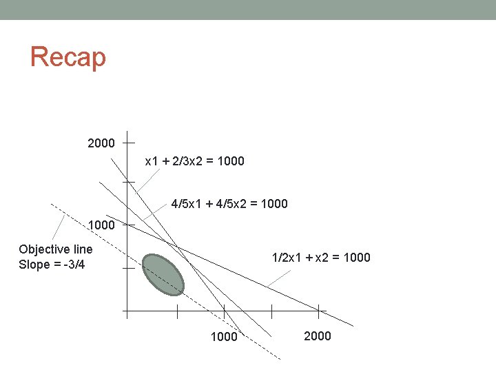
Recap 2000 x 1 + 2/3 x 2 = 1000 4/5 x 1 + 4/5 x 2 = 1000 Objective line Slope = -3/4 1/2 x 1 + x 2 = 1000 2000

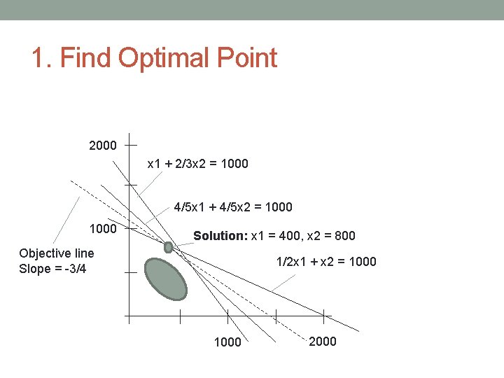
1. Find Optimal Point 2000 x 1 + 2/3 x 2 = 1000 4/5 x 1 + 4/5 x 2 = 1000 Solution: x 1 = 400, x 2 = 800 Objective line Slope = -3/4 1/2 x 1 + x 2 = 1000 2000

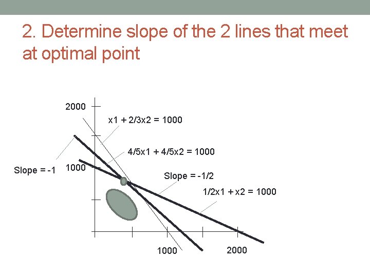
2. Determine slope of the 2 lines that meet at optimal point 2000 x 1 + 2/3 x 2 = 1000 4/5 x 1 + 4/5 x 2 = 1000 Slope = -1/2 1/2 x 1 + x 2 = 1000 2000

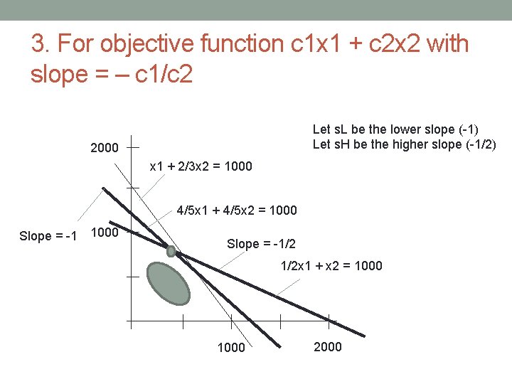
3. For objective function c 1 x 1 + c 2 x 2 with slope = – c 1/c 2 Let s. L be the lower slope (-1) Let s. H be the higher slope (-1/2) 2000 x 1 + 2/3 x 2 = 1000 4/5 x 1 + 4/5 x 2 = 1000 Slope = -1/2 1/2 x 1 + x 2 = 1000 2000

3. For objective function c 1 x 1 + c 2 x 2 with slope = – c 1/c 2 Let s. L be the lower slope (-1) Let s. H be the higher slope (-1/2) 2000 x 1 + 2/3 x 2 = 1000 4/5 x 1 + 4/5 x 2 = 1000 Slope = -1 1000 a) Range for c 1. Fix c 2 and solve for c 1 -c 1/c 2 >= s. L -c 1/c 2 <= s. H Slope = -1/2 1/2 x 1 + x 2 = 1000 2000

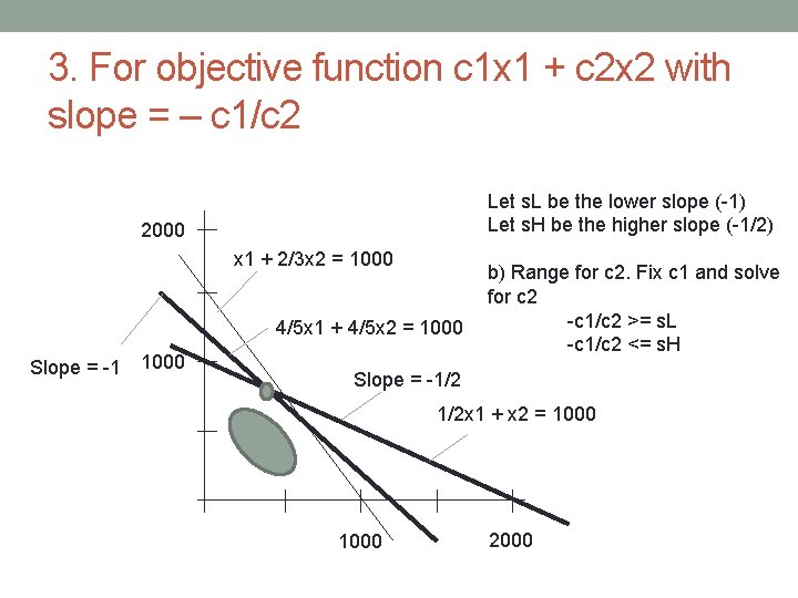
3. For objective function c 1 x 1 + c 2 x 2 with slope = – c 1/c 2 Let s. L be the lower slope (-1) Let s. H be the higher slope (-1/2) 2000 x 1 + 2/3 x 2 = 1000 4/5 x 1 + 4/5 x 2 = 1000 Slope = -1 1000 b) Range for c 2. Fix c 1 and solve for c 2 -c 1/c 2 >= s. L -c 1/c 2 <= s. H Slope = -1/2 1/2 x 1 + x 2 = 1000 2000

Sensitivity Analysis - LINDO • Consider the Cross. Chek hockey stick production problem: • Consider two high-end hockey sticks, A and B. $150 and $200 profit are earned from each sale of A and B, respectively. Each product goes through 3 phases of production. • A requires 1 hour of work in phase 1, 48 min in phase 2, and 30 min in phase 3. • B requires 40 min, 48 min and 1 hour, respectively. • Limited manufacturing capacity: • phase 1 1000 total hours • phase 2 960 • phase 3 1000 • How many of each product should be produced? • Maximize profit • Satisfy constraints. Max s. t 150 x 1 + 200 x 2 x 1 + 2/3 x 2 <= 1000 4/5 x 1 + 4/5 x 2 <= 960 1/2 x 1 + x 2 <= 1000 x 1, x 2 >= 0 • Management believes that Cross. Chek might only receive $120 profit from the sale of each lower-profit hockey stick. Will that affect the optimal solution? What about a (separate) change in the profit from higher-profit sticks to $125?

Caveat • We know that changing the coefficient of x 1 in the objective function 150 x 1 + 200 x 2 from 150 to 120 does not change the solution • We know that changing the coefficient of x 2 in the objective function 150 x 1 + 200 x 2 from, say 200 to 175 does not change the solution • However, these ranges are only valid when the other coefficient remains fixed • Changing both simultaneously may or may not change the optimal solution

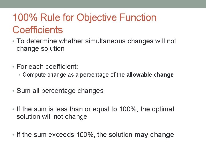
100% Rule for Objective Function Coefficients • To determine whether simultaneous changes will not change solution • For each coefficient: • Compute change as a percentage of the allowable change • Sum all percentage changes • If the sum is less than or equal to 100%, the optimal solution will not change • If the sum exceeds 100%, the solution may change

Sensitivity Analysis • Consider the Cross. Chek hockey stick production problem: • Consider two high-end hockey sticks, A and B. $150 and $200 profit are earned from each sale of A and B, respectively. Each product goes through 3 phases of production. • A requires 1 hour of work in phase 1, 48 min in phase 2, and 30 min in phase 3. • B requires 40 min, 48 min and 1 hour, respectively. • Limited manufacturing capacity: • phase 1 1000 total hours • phase 2 960 • phase 3 1000 • How many of each product should be produced? • Maximize profit • Satisfy constraints. Max s. t 150 x 1 + 200 x 2 x 1 + 2/3 x 2 <= 1000 4/5 x 1 + 4/5 x 2 <= 960 1/2 x 1 + x 2 <= 1000 x 1, x 2 >= 0 • Management believes that Cross. Chek might only receive $120 profit from the sale of each lower-profit hockey stick. Will that affect the optimal solution? What about a (separate) change in the profit from higher-profit sticks to $125?

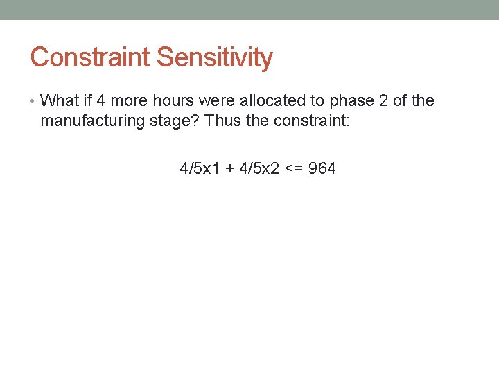
Constraint Sensitivity • What if 4 more hours were allocated to phase 2 of the manufacturing stage? Thus the constraint: 4/5 x 1 + 4/5 x 2 <= 964

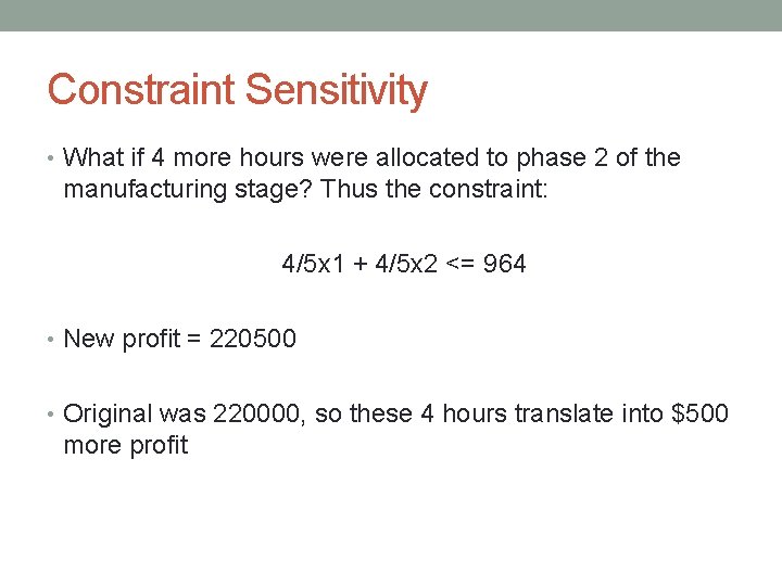
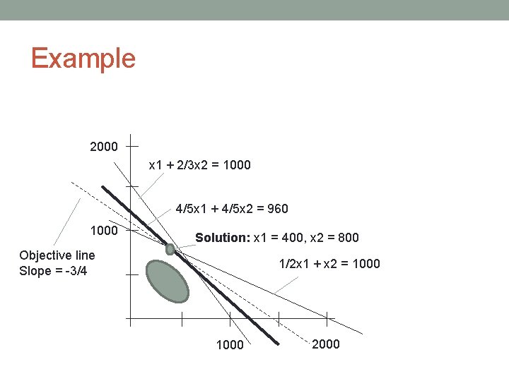
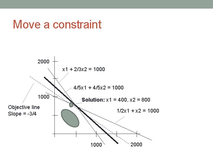
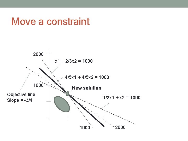
Constraint Sensitivity • What if 4 more hours were allocated to phase 2 of the manufacturing stage? Thus the constraint: 4/5 x 1 + 4/5 x 2 <= 964 • New profit = 220500 • Original was 220000, so these 4 hours translate into $500 more profit

Constraint Sensitivity • What if 8 more hours were allocated to phase 2 of the manufacturing stage? Thus the constraint: 4/5 x 1 + 4/5 x 2 <= 968

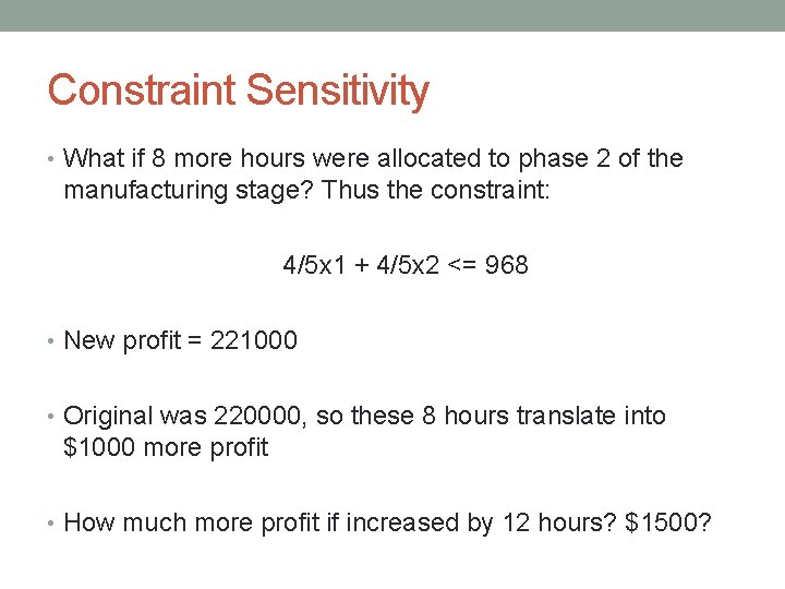
Constraint Sensitivity • What if 8 more hours were allocated to phase 2 of the manufacturing stage? Thus the constraint: 4/5 x 1 + 4/5 x 2 <= 968 • New profit = 221000 • Original was 220000, so these 8 hours translate into $1000 more profit • How much more profit if increased by 12 hours? $1500?

Example 2000 x 1 + 2/3 x 2 = 1000 4/5 x 1 + 4/5 x 2 = 960 1000 Solution: x 1 = 400, x 2 = 800 Objective line Slope = -3/4 1/2 x 1 + x 2 = 1000 2000

Move a constraint 2000 x 1 + 2/3 x 2 = 1000 4/5 x 1 + 4/5 x 2 = 1000 Solution: x 1 = 400, x 2 = 800 Objective line Slope = -3/4 1/2 x 1 + x 2 = 1000 2000

Move a constraint 2000 x 1 + 2/3 x 2 = 1000 4/5 x 1 + 4/5 x 2 = 1000 New solution Objective line Slope = -3/4 1/2 x 1 + x 2 = 1000 2000

Dual Prices • The dual price of a constraint is the improvement in the optimal solution, per unit increase in the right-hand side value of the constraint. The dual price of the processor configuration constraint is thus $500/4 = $125. • A negative dual price indicates how much worse the optimal solution will get with each unit increase in the right -hand side value of the constraint

Move a constraint 2000 x 1 + 2/3 x 2 = 1000 4/5 x 1 + 4/5 x 2 = 1000 New solution Objective line Slope = -3/4 1/2 x 1 + x 2 = 1000 2000

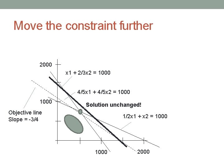
Move the constraint further 2000 x 1 + 2/3 x 2 = 1000 4/5 x 1 + 4/5 x 2 = 1000 Solution unchanged! Objective line Slope = -3/4 1/2 x 1 + x 2 = 1000 2000

Range of Feasibility • The dual price may only be applicable for small increases. Large increases may result in a change in the optimal extreme point, and thus increasing this value further may not have the same effect. • The range of values the right-hand side can take without affecting the dual price is called the range of feasibility. This is similar to the concept of range of optimality for objective function coefficients. There is no easy way to manually calculate these ranges, but they can be found under the RIGHT HAND SIDE RANGES heading in LINDO.

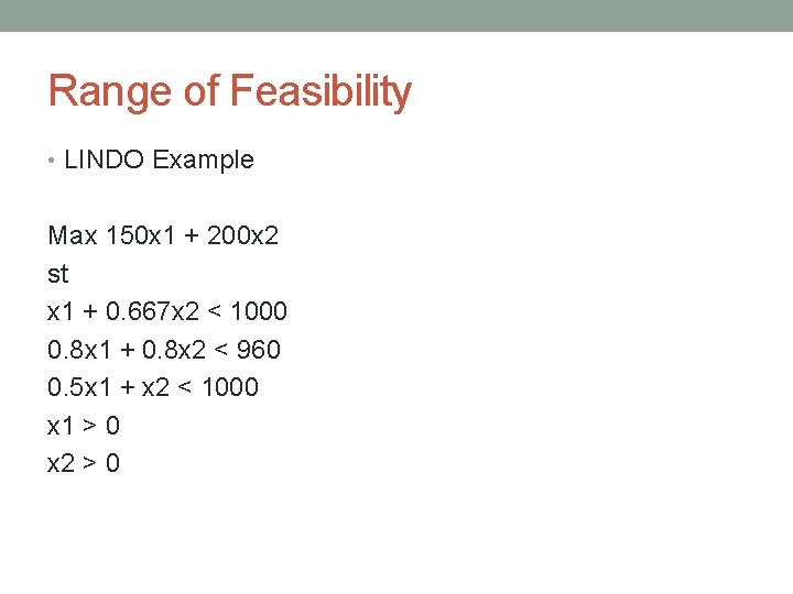
Range of Feasibility • LINDO Example Max 150 x 1 + 200 x 2 st x 1 + 0. 667 x 2 < 1000 0. 8 x 1 + 0. 8 x 2 < 960 0. 5 x 1 + x 2 < 1000 x 1 > 0 x 2 > 0